impulseplot

R2026b

Plot impulse response of dynamic system

Syntax

impulseplot(sys)

impulseplot(sys1,sys2,...,sysN)

impulseplot(sys1,LineSpec1,...,sysN,LineSpecN)

impulseplot(___,t)

impulseplot(sys,t,p)

impulseplot(___,plotoptions)

impulseplot(___,Name=Value)

ip = impulseplot(parent,___)

ip = impulseplot(___)

Description

The impulseplot function plots the impulse response of a dynamic system model. To customize the plot, you can return an ImpulsePlot object and modify it using dot notation. For more information, see Customize Linear Analysis Plots at Command Line (Control System Toolbox).

To obtain impulse response data or create an impulse plot with default plotting options, use the impulse function.

impulseplot(sys) plots the impulse response of the dynamic system model sys.

If sys is a multi-input, multi-output (MIMO) model, then the impulseplot function creates a grid of plots with each plot displaying the impulse response of one input-output pair.

If sys is a model with complex coefficients, then the plot shows both the real and imaginary components of the response on a single axes and indicates the imaginary component with a diamond marker. You can also view the response using magnitude-phase and complex-plane plots. (since R2025a)

impulseplot(sys1,sys2,...,sysN) plots the impulse response of multiple dynamic systems sys1,sys2,…,sysN on the same plot.

impulseplot(sys1,LineSpec1,...,sysN,LineSpecN) sets the line style, marker type, and color for the impulse response of each specified system.

impulseplot(___,t) simulates the response for the time steps specified by t. You can use t with any of the input argument combinations in previous syntaxes. To define the time steps, you can specify:

• Final simulation time using a scalar value.

• The initial and final simulation times using a two-element vector. (since R2023b)

• All the time steps using a vector.

impulseplot(sys,t,p) also specifies the parameter trajectory p for LPV models. (since R2023a)

impulseplot(___,plotoptions) plots the impulse response with the plotting options specified in plotoptions. Settings you specify in plotoptions override the plotting preferences for the current MATLAB^® session. This syntax is useful when you want to write a script to generate multiple plots that look the same regardless of the local preferences.

impulseplot(___,Name=Value) specifies response properties using one or more name-value arguments. For example, impulseplot(sys,LineWidth=1) sets the plot line width to 1. (since R2026a)

• When plotting responses for multiple systems, the specified name-value arguments apply to all responses.

• The following name-value arguments override values specified in other input arguments.

  • Time — Overrides time values specified using t

  • Parameter — Overrides parameter values specified using p

  • Color — Overrides colors specified using LineSpec

  • MarkerStyle — Overrides marker styles specified using LineSpec

  • LineStyle — Overrides line styles specified using LineSpec

ip = impulseplot(parent,___) plots the impulse response in the specified parent graphics container, such as a Figure or TiledChartLayout, and sets the Parent property. Use this syntax when you want to create a plot in a specified open figure or when creating apps in App Designer.

ip = impulseplot(___) plots the impulse response and returns the corresponding chart object. To customize the appearance and behavior of the response plot, modify the chart object properties using dot notation.

Examples

Customize Impulse Plot Using Chart Object

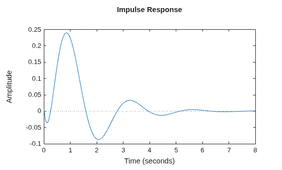
Generate a random state-space model with 5 states and create the impulse response plot with chart object ip.

rng("default")
sys = rss(5);
ip = impulseplot(sys);

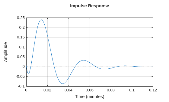
Change the time units to minutes and turn on the grid.

ip.TimeUnit = "minutes";
grid on

The impulse plot automatically updates when you modify the chart object properties.

Impulse Plot with Specified Grid Color

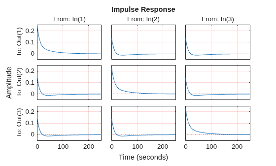
For this example, consider a MIMO state-space model with 3 inputs, 3 outputs and 3 states. Create an impulse plot with red colored grid lines.

Create the MIMO state-space model sys_mimo.

J = [8 -3 -3; -3 8 -3; -3 -3 8];
F = 0.2*eye(3);
A = -J\F;
B = inv(J);
C = eye(3);
D = 0;
sys_mimo = ss(A,B,C,D);
size(sys_mimo)

State-space model with 3 outputs, 3 inputs, and 3 states.

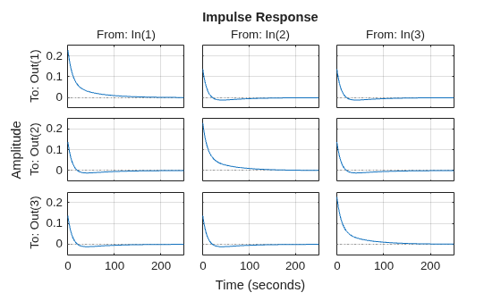
Create an impulse plot with chart object ip and display the grid.

ip = impulseplot(sys_mimo);
grid on

Set the grid color to red.

ip.AxesStyle.GridColor = [1 0 0];

The impulse plot automatically updates when you modify the chart object. For MIMO models, impulseplot produces a grid of plots, each plot displaying the impulse response of one I/O pair.

Plot Impulse Responses of Identified Models with Confidence Region

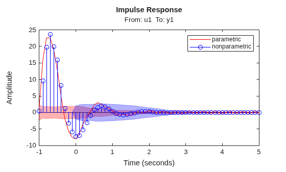
Compare the impulse response of a parametric identified model to a nonparametric (empirical) model, and view their 3-σ confidence regions. (Identified models require System Identification Toolbox™ software.)

Identify a parametric and a nonparametric model from sample data.

load iddata1 z1
sys1 = ssest(z1,4); 
sys2 = impulseest(z1);

Plot the impulse responses of both identified models. Use the plot handle to display the 3-σ confidence regions.

t = -1:0.1:5;
h = impulseplot(sys1,'r',sys2,'b',t);
showConfidence(h,3)
legend('parametric','nonparametric')

The nonparametric model sys2 shows higher uncertainty.

Customized Impulse Response Plot at Specified Time

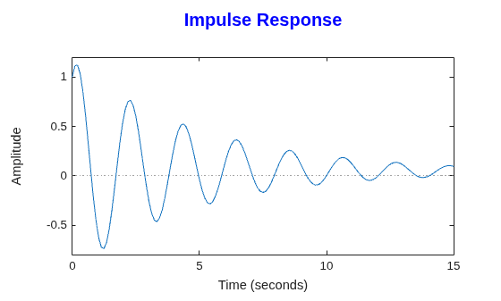
For this example, examine the impulse response of the following zero-pole-gain model and limit the impulse plot to tFinal = 15 s. Use 15-point blue text for the title.

sys = zpk(-1,[-0.2+3j,-0.2-3j],1)*tf([1 1],[1 0.05]);
tFinal = 15;

Create the impulse response plot and specify the title size and color.

ip = impulseplot(sys,tFinal);
ip.Title.FontSize = 15;
ip.Title.Color = [0 0 1];

Impulse Response of Model with Complex Coefficients

Since R2025a

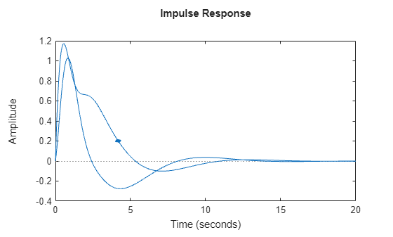
Create a state-space model with complex coefficients.

A = [-2-2i -2;1 0];
B = [2;0];
C = [0 0.5+2.5i];
D = 0;
sys = ss(A,B,C,D);

Plot the impulse response of the system.

ip = impulseplot(sys);

By default, the plot shows the real and imaginary components of the response on a single axes, indicating the imaginary component using a diamond marker.

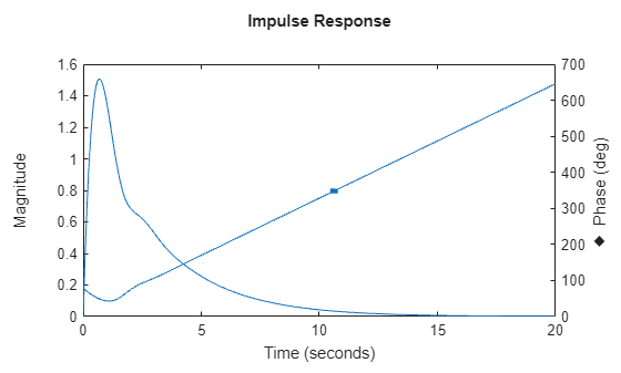
You can also view the complex response using either a magnitude-phase plot or a complex-plane plot. For example, to view the magnitude and phase of the response, right-click the plot area and select Complex View >Magnitude-Phase.

ip.ComplexViewType = "magnitudephase";

The plot shows the magnitude and phase of the response on a single axes, indicating the phase plot using a diamond marker.

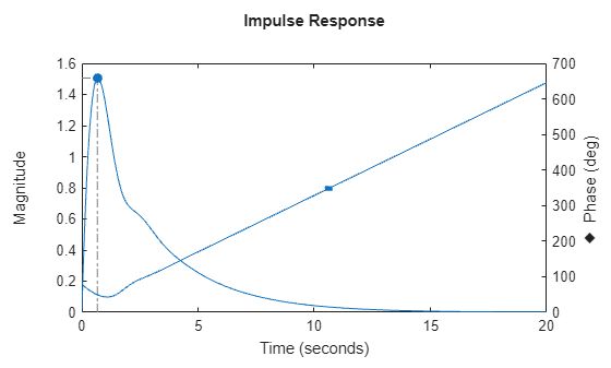
You can view response characteristics in the plot. For example, to view the peak response, right-click the plot and select Characteristics > Peak Response.

Alternatively, you can enable the Visible property of the corresponding characteristic parameter of the chart object.

ip.Characteristics.PeakResponse.Visible = "on";

Input Arguments

sys — Dynamic system

dynamic system model | model array

Dynamic system, specified as a SISO or MIMO dynamic system model or an array of dynamic system models. You can use these types of dynamic systems:

• Continuous-time or discrete-time numeric LTI models, such as tf, zpk, or ss models.

• Generalized or uncertain LTI models such as genss or uss models. (Using uncertain models requires Robust Control Toolbox™ software.)

  • For tunable control design blocks, the function evaluates the model at its current value for both plotting and returning response data.

  • For uncertain control design blocks, the function plots the nominal value and random samples of the model. When you use output arguments, the function returns response data for the nominal model only.

• Sparse state-space models such as sparss and mechss models.

• Identified LTI models, such as idtf, idss, or idproc models. For such models, the function can also plot confidence intervals and return standard deviations of the frequency response. See Step Responses of Identified Models with Confidence Regions.

• Linear time-varying (ltvss (Control System Toolbox)) and linear parameter-varying (lpvss (Control System Toolbox)) models.

This function does not support frequency-response data models such as frd, genfrd, or idfrd models.

If sys is an array of models, the function plots the responses of all models in the array on the same axes. See Step Response of Systems in a Model Array.

LineSpec — Line style, marker, and color

string | character vector

Line style, marker, and color, specified as a string or character vector containing symbols. The symbols can appear in any order. You do not need to specify all three characteristics. For example, specify the marker and omit the line style, then the plot shows only the marker and no line.

Example: '--or' is a red dashed line with circle markers.

Line Style	Description
"-"	Solid line
"--"	Dashed line
":"	Dotted line
"-."	Dash-dotted line

Marker	Description
"o"	Circle
"+"	Plus sign
"*"	Asterisk
"."	Point
"x"	Cross
"_"	Horizontal line
"|"	Vertical line
"s"	Square
"d"	Diamond
"^"	Upward-pointing triangle
"v"	Downward-pointing triangle
">"	Right-pointing triangle
"<"	Left-pointing triangle
"p"	Pentagram
"h"	Hexagram

Color	Description
"r"	red
"g"	green
"b"	blue
"c"	cyan
"m"	magenta
"y"	yellow
"k"	black
"w"	white

t — Time steps

positive scalar | two-element vector | vector | []

Time steps at which to compute the response, specified as one of these values:

• Positive scalar tFinal— Compute the response from t = 0 to t = tFinal.

• Two-element vector [t0 tFinal] — Compute the response from t = t0 to t = tFinal. (since R2023b)

• Vector Ti:dt:Tf— Compute the response for the time points specified in t.

  • For continuous-time systems, dt is the sample time of a discrete approximation to the continuous system.

  • For discrete-time systems with a specified sample time, dt must match the sample time property Ts of sys.

  • For discrete-time systems with an unspecified sample time (Ts = -1), dt must be 1.

• [] — Automatically select time values based on system dynamics.

When you specify a time range using either tFinal or [t0 tFinal]:

• For continuous-time systems, the function automatically determines the size of the time step and number of points based on the system dynamics.

• For discrete-time systems with a specified sample time, the function uses the sample time of sys as the step size.

• For discrete-time systems with unspecified sample time (Ts = -1), the function interprets tFinal as the number of sampling periods to simulate with a sample time of 1 second.

Express t using the time units specified in the TimeUnit property of sys.

Before R2026a: Specify time values using the Responses.SourceData.TimeSpec property.

Before R2026b: This property is called TimeSpec.

p — LPV model parameter trajectory

matrix | function handle

LPV model parameter trajectory, specified as a matrix or a function handle.

• For exogenous or explicit trajectories, specify p as a matrix with dimensions N-by-Np, where N is the number of time samples and Np is the number of parameters.

  Thus, the row vector p(i,:) contains the parameter values at the ith time step.

• For endogenous or implicit trajectories, specify p as a function handle of the form p = F(t,x,u) in continuous time and p = F(k,x,u) in discrete time that gives parameters as a function of time t or time sample k, state x, and input u. For implicit trajectories, you must specify an initial condition for the simulation.

  This option is useful when you want to simulate quasi-LPV models.

plotoptions — Time response plot options

timeoptions object

Time response plot options, specified as a timeoptions (Control System Toolbox) object. You can use these options to customize the plot appearance. Settings you specify in plotoptions override the preference settings for the current MATLAB session.

parent — Parent graphics container

Figure object | TiledChartLayout object | UIFigure object | UIGridLayout object | UIPanel object | UITab object

Parent graphics container, specified as one of these objects:

• Figure

• TiledChartLayout

• UIFigure

• UIGridLayout

• UIPanel

• UITab

Name-Value Arguments

Specify optional pairs of arguments as Name1=Value1,...,NameN=ValueN, where Name is the argument name and Value is the corresponding value. Name-value arguments must appear after other arguments, but the order of the pairs does not matter.

Example: impulseplot(sys,LegendDisplay="off") hides the response of sys from the plot legend.

Response Computation

Time — Time values

scalar | vector | []

Time steps at which to compute the response, specified as one of these values. Specifying time values using a name-value argument overrides the time values that you specify using t.

• Positive scalar tFinal— Compute the response from t = 0 to t = tFinal.

• Two-element vector [t0 tFinal] — Compute the response from t = t0 to t = tFinal.

• Vector Ti:dt:Tf— Compute the response for the time points specified in t.

  • For continuous-time systems, dt is the sample time of a discrete approximation to the continuous system.

  • For discrete-time systems with a specified sample time, dt must match the sample time property Ts of sys.

  • For discrete-time systems with an unspecified sample time (Ts = -1), dt must be 1.

• [] — Automatically select time values based on system dynamics.

When you specify a time range using either tFinal or [t0 tFinal]:

• For continuous-time systems, the function automatically determines the size of the time step and number of points based on the system dynamics.

• For discrete-time systems with a specified sample time, the function uses the sample time of sys as the step size.

• For discrete-time systems with unspecified sample time (Ts = -1), the function interprets tFinal as the number of sampling periods to simulate with a sample time of 1 second.

Express Time using the time units specified in the TimeUnit property of sys.

Parameter — LPV model parameter trajectory

matrix | function handle

LPV model parameter trajectory, specified as a matrix or a function handle. Specifying parameter values using a name-value argument overrides the parameter values that you specify using p.

• For exogenous or explicit trajectories, specify Parameter as a matrix with dimensions N-by-Np, where N is the number of time samples and Np is the number of parameters.

  Thus, the row vector p(i,:) contains the parameter values at the ith time step.

• For endogenous or implicit trajectories, specify Parameter as a function handle of the form p = F(t,x,u) in continuous time and p = F(k,x,u) in discrete time that gives parameters as a function of time t or time sample k, state x, and input u. For implicit trajectories, you must specify an initial condition for the simulation.

  This option is useful when you want to simulate quasi-LPV models.

Amplitude — Input level change

1 (default) | scalar | vector

Since R2026b

Input level change relative to the input signal bias, specified as a scalar or vector.

• For single-input systems, Amplitude is a scalar value.

• For multi-input systems, Amplitude is a vector of length N _u, where N _u is the number of input channels. Each vector value corresponds to the level change amplitude in that input channel. The functions compute the responses one input channel at a time.

Complex Number Support: Yes

Bias — Baseline input signal value

0 (default) | scalar | vector | "u0"

Since R2026b

Baseline input signal value, specified as a scalar or vector.

• For single-input systems, Bias is a scalar value.

• For multi-input systems, Bias is a vector of length N _u, where N _u is the number of input channels. Each vector value corresponds to the signal value in that input channel. The functions compute the responses one input channel at a time.

• For state-space models with offsets, set Bias = "u0" to apply the step or impulse change relative to the model offsets u ₀, u ₀(t) of the LTV model, or u ₀(t,p) of the LPV model. For LTV and LPV models, this is the u0 output of the data function. The total input signal is then u ₀ + u(t).

Delay — Input signal delay

0 (default) | nonnegative scalar

Since R2026b

Input signal delay, specified as a nonnegative scalar value. This value specifies when the change occurs relative to the simulation start time T ₀.

InitialCondition — Initial condition

[] (default) | vector | "x0" | operating condition created using findop | initialCondition object

Since R2026b

Initial condition, specified as one of these values:

• [] — Start simulation from the steady-state condition for the input value specified in Bias. For state-space models without internal delays, the initial state x_init is the solution to the following, where U is the Bias value:

  • Continuous time — 0 = A x_init + B U

  • Discrete time — x_init = A x_init + B U

• Vector of initial state values with length equal to the number of states in the model — Start simulation from the specified initial state and use Bias as the initial input value.

• "x0" — Use Bias as the initial input value and evaluate state offset value x ₀ for state-space models, x ₀(T ₀) for LTV models, or x ₀(T ₀,p(T ₀)) for LPV models. For LTV and LPV models, the state offset value is the x0 output of the data function evaluated at t = T ₀.

• initialCondition object for identified models (requires System Identification Toolbox™ software) — Start simulation from the specified initial state and use Bias as the initial input value.

• Operating condition created using findop (Control System Toolbox) — An operating point object allows you to start the simulation from a steady-state operating condition with nonzero past u, w, and y values. When you specify an operating point object, the value of Bias is ignored.

Response Style

Name — Response name

string | character vector

Response name, specified as a string or character vector and stored as a string.

Visible — Response visibility

"on" (default) | on/off logical value

Response visibility, specified as one of these logical on/off values:

• "on", 1, or true — Display the response in the plot.

• "off", 0, or false — Do not display the response in the plot.

The value is stored as an on/off logical value of type matlab.lang.OnOffSwitchState.

LegendDisplay — Option to list response in legend

"on" (default) | on/off logical value

Option to list the response in the legend, specified as one of these logical on/off values:

• "on", 1, or true — List the response in the legend.

• "off", 0, or false — Do not list the response in the legend.

The value is stored as an on/off logical value of type matlab.lang.OnOffSwitchState.

MarkerStyle — Marker style

"none" | "o" | "+" | "*" | "." | ...

Marker style, specified as one of these values. Specifying a marker style using a name-value argument overrides any marker style that you specify using LineSpec.

Marker	Description
"none"	No marker
"o"	Circle
"+"	Plus sign
"*"	Asterisk
"."	Point
"x"	Cross
"_"	Horizontal line
"|"	Vertical line
"s"	Square
"d"	Diamond
"^"	Upward-pointing triangle
"v"	Downward-pointing triangle
">"	Right-pointing triangle
"<"	Left-pointing triangle
"p"	Pentagram
"h"	Hexagram

Color — Plot color

RGB triplet | hexadecimal color code | color name

Plot color, specified as an RGB triplet or a hexadecimal color code and stored as an RGB triplet. Specifying a color using a name-value argument overrides any color that you specify using LineSpec.

You can also specify some common colors by name. This table lists these colors and their corresponding RGB triplets and hexadecimal color codes.

Color Name	RGB Triplet	Hexadecimal Color Code
"red" or "r"	[1 0 0]	#FF0000
"green" or "g"	[0 1 0]	#00FF00
"blue" or "b"	[0 0 1]	#0000FF
"cyan" or "c"	[0 1 1]	#00FFFF
"magenta" or "m"	[1 0 1]	#FF00FF
"yellow" or "y"	[1 1 0]	#FFFF00
"black" or "k"	[0 0 0]	#000000
"white" or "w"	[1 1 1]	#FFFFFF

LineStyle — Line style

"-" | "--" | ":" | "-."

Line style, specified as one of these values. Specifying a line style using a name-value argument overrides any line style that you specify using LineSpec.

Line Style	Description
"-"	Solid line
"--"	Dashed line
":"	Dotted line
"-."	Dash-dotted line
"none"	No line

MarkerSize — Marker size

positive scalar

Marker size, specified as a positive scalar.

LineWidth — Line width

positive scalar

Line width, specified as a positive scalar.

SeriesIndex — Series index

positive integer | "none"

Series index, specified as a positive integer or "none".

By default, the SeriesIndex property is a number that corresponds to the order in which the response was added to the chart, starting at 1. MATLAB uses the number to calculate indices for automatically assigning color, line style, or markers for responses. Any responses in the chart that have the same SeriesIndex number also have the same color, line style, and markers.

A SeriesIndex value of "none" indicates that a response does not participate in the indexing scheme.

Output Arguments

ip — Chart object

ImpulsePlot object

Chart object, returned as a ImpulsePlot object. To customize your plot appearance and behavior, modify the properties of this object using dot notation. For more information, see ImpulsePlot Properties (Control System Toolbox).

Version History

Introduced in R2012a

R2026b: Specify response computation options new properties and name-value arguments

You can now specify response options using these name-value arguments

• Bias — Baseline input signal value

• Amplitude — Input level change

• Delay — Input signal delay

• InitialCondition — System initial condition

These arguments replace response configuration using a RespConfig object. For more information, see Setting response options using RespConfig object not recommended.

R2026b: Setting response options using RespConfig object not recommended

Setting response options using a RespConfig object is not recommended. Use the Bias, Amplitude, Delay, and InitialCondition name-value arguments instead.

This table shows some uses of RespConfig and how to update your code to use the new name-value arguments. Here, sysLPV is a linear parameter-varying model.

Not Recommended	Recommended
config = RespConfig( ... Amplitude=0.5, ... Bias=1, ... Delay=2, ... InitialState=[1 2 3]); impulseplot(sys,config)	impulseplot(sys, ... Amplitude=0.5, ... Bias=1, ... Delay=2, ... InitialCondition=[1 2 3])
config = RespConfig( ... Bias=-1, ... InitialParameter=pinit); impulseplot(sysLPV,t,pFcn,config)	IC = findop(sysLPV,t(1),pinit,u=-1); impulseplot(sysLPV,t,pFcn,InitialCondition=IC)
For LPV systems with state offsets: config = RespConfig( ... InitialState="x0", ... InitialParameter=pinit) impulseplot(sysLPV,t,pFcn,config)	[~,~,~,~,~,~,x0] = sysLPV.DataFunction(t(1),pinit); impulseplot(sysLPV,t,pFcn,InitialCondition=x0)
For LPV systems with input offsets: config = RespConfig( ... Bias="u0", ... InitialParameter=pinit) impulseplot(sysLPV,t,pFcn,config)	[~,~,~,~,~,~,~,u0] = sysLPV.DataFunction(t(1),pinit); IC = findop(sysLPV,tinit,pinit,u=u0); impulseplot(sysLPV,t,pFcn,InitialCondition=IC)

R2026a: Specify response properties using name-value arguments

You can now specify response properties using name-value arguments.

When plotting responses for multiple systems, the specified property values apply to all responses.

If a name-value argument sets the same property as another input argument, the property value is set to the name-value argument.

R2026a: Support for sparse index-2 models

Starting in R2026a, the impulseplot function supports sparse index-2 DAEs.

R2026a: Specifying axes object as parent not recommended

Specifying an Axes object or a UIAxes object as the parent container of a linear analysis plot is not recommended. Instead, specify the parent container as one of these objects:

• Figure

• TiledChartLayout

• UIFigure

• UIGridLayout

• UIPanel

• UITab

R2025a: Support for dynamic systems with complex coefficients

Starting in R2025a, the impulseplot function supports dynamic systems with complex coefficients. You can plot the response for a complex system as:

• Real and imaginary responses on a single axis

• Magnitude and phase responses on a single axis

• A single response on a complex plane

R2024b: Improved customization workflows and integration with MATLAB plotting tools

Starting in R2024b, the impulseplot function returns an ImpulsePlot chart object. Previously, the impulseplot function returned a handle to the resulting plot.

The new chart object allows you to customize your plot using dot notation.

The new chart object also improves integration with MATLAB plotting tools. For example:

• You can now add impulse plots to tiled chart layouts.

• Saving and loading a parent figure now maintains full plot interactivity.

• You can add a response to your impulse plot using the new addResponse function.

The following functionality changes might require updates to your code:

• The gca function now returns the chart object rather than an axes within the plot.

• You can no longer access the graphics objects within an impulse plot using the Children property of its parent figure.