Building Nonlinear ARX Models with Nonlinear and Custom Regressors
This example shows how to use polynomial and custom regressors in Nonlinear ARX (IDNLARX) models.
Introduction
In an IDNLARX model, each output is a function of regressors which are transformations of past inputs and past outputs. Typical regressors are simply delayed input or output variables represented by the linearRegressor specification object, or polynomials of the delayed variables represented by the polynomialRegressor object. However, other than the ability to impose absolute value (e.g., abs(y(t-1))), you cannot create complex mathematical formulas using these types of regressors. For example, if your output function requires a regressor of the form sin(u(t-3)).*exp(-abs(u(t))), you need a way to type-in your custom formula in the expression for the regressor. This is facilitated by the customRegressor objects. As the name suggests, you use the customRegressor object to incorporate arbitrary, custom formulas as regressors for your Nonlinear ARX model.
Consider the example of an electric system with both the voltage V and the current I as inputs. If it is known that the electric power is an important quantity of the system, then it makes sense to form the custom regressor V*I. It may be more efficient to use appropriately defined custom regressors than to use the linear and polynomial regressors only.
SISO Example: Modeling an Internal Combustion Engine
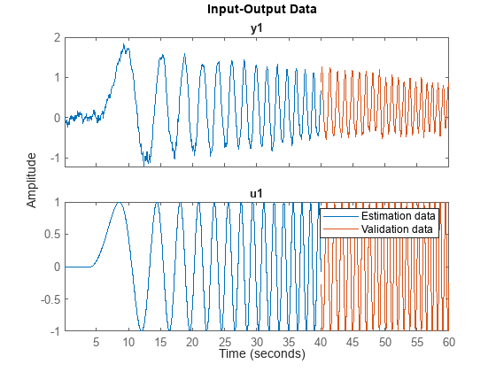
The file icEngine.mat contains one data set with 1500 input-output samples collected at the a sampling rate of 0.04 seconds. The input u(t) is the voltage [V] controlling a By-Pass Idle Air Valve (BPAV), and the output y(t) is the engine speed [RPM/100]. The data is loaded and split into a dataset ze for model estimation and another dataset zv for model validation.
load icEngine
z = iddata(y,u,0.04);
ze = z(1:1000);
zv = z(1001:1500);
plot(ze,zv)
legend('Estimation data','Validation data')
Linear Regressors as ARX Orders
Order matrix [na nb nk], which is also used in the linear ARX model, help easily define the linear regressors, which are simply the input/output variables delayed by certain number of samples. The choice of model orders requires trial and error. For this example let us use [na nb nk] = [4 2 10], corresponding to the linear regressors y(t-1), y(t-2), y(t-3), y(t-4), u(t-10), u(t-11). Choose a linear output function, so that the model output is just a weighted sum of its six regressors, plus an offset.

sys0 = nlarx(ze, [4 2 10], idLinear);
The input name, output name and the list of regressors of this model are displayed below. Notice that the default names 'u1', 'y1' are used.
sys0.InputName
ans = 1×1 cell array
    {'u1'}
sys0.OutputName
ans = 1×1 cell array
    {'y1'}
disp(getreg(sys0))
    {'y1(t-1)' }
    {'y1(t-2)' }
    {'y1(t-3)' }
    {'y1(t-4)' }
    {'u1(t-10)'}
    {'u1(t-11)'}
These are linear regressors. They are stored in the model's Regressors property as a linearRegressor object.
sys0.Regressors
ans =
Linear regressors in variables y1, u1
       Variables: {'y1'  'u1'}
            Lags: {[1 2 3 4]  [10 11]}
     UseAbsolute: [0 0]
    TimeVariable: 't'

  Regressors described by this set
The "Regressors" property stores the information on the regressor implicitly using a regression specification object. You can think of the order matrix [4 2 10] as a shortcut way of specifying linear regressors, where are lags are contiguous and minimum lag in the output variable is fixed to 1.
Linear Regressors Using linearRegressor Specification Object
A more flexible way that allows picking of variables with arbitrary lags is to use the linearRegressor object. In the above configuration, the variable y1 has lags [1 2 3 4], while the variable u1 has lags [10 11]. Using a linearRegressor object, the same configuration can be achieved as follows:
LinReg = linearRegressor({'y1','u1'}, {1:4, [10, 11]});
sys1 = nlarx(ze, LinReg, idLinear)
sys1 = Nonlinear ARX model with 1 output and 1 input Inputs: u1 Outputs: y1 Regressors: Linear regressors in variables y1, u1 List of all regressors Output function: Linear with offset Sample time: 0.04 seconds Status: Estimated using NLARX on time domain data "ze". Fit to estimation data: 94.35% (prediction focus) FPE: 0.001877, MSE: 0.00183 Model Properties
Compare the estimation syntaxes of the models sys1 and sys0; when creating sys1 you replaced the order matrix with a linear regressor specification object. The resulting models sys0 and sys1 are identical.
[getpvec(sys0), getpvec(sys1)] % estimated parameter vectors of sys0 and sys1ans = 7×2
0.7528 0.7528
0.0527 0.0527
-0.0621 -0.0621
-0.0425 -0.0425
-0.0165 -0.0165
-0.0289 -0.0289
-0.0000 -0.0000
You will use the linearRegressor object to specify the regressors in place of the order matrix, in the following scenarios:
you want to use arbitrary (non-contiguous) lags in variables such as the set
you want the minimum lag in the output variable(s) to be different than 1, for example, the set
you want to use absolute values of the variables such as in the set where only the absolute value of variable 'y1' is used. This can be achieved by doing
LinRegWithAbs = linearRegressor({'y1','u1'},{[1 10], [0 2]},[true, false])LinRegWithAbs =
Linear regressors in variables y1, u1
Variables: {'y1' 'u1'}
Lags: {[1 10] [0 2]}
UseAbsolute: [1 0]
TimeVariable: 't'
Regressors described by this set
Polynomial Regressors
Often regressors that are polynomials of delayed I/O variables are required. These can be added to the model using the polynomialRegressor object. Suppose you want to add , as regressors to the model. You first create a specification object with these settings and then add this object to the model.
% Create order 2 regressors in variables 'u1' and 'y1', with lags 10 and 1
% respectively
PolyReg = polynomialRegressor({'u1','y1'},{10, 1},2);

% Use LinReg and PolyReg in the model
sys2 = nlarx(ze, [LinReg; PolyReg], idLinear)
sys2 =

Nonlinear ARX model with 1 output and 1 input
  Inputs: u1
  Outputs: y1

Regressors:
  1. Linear regressors in variables y1, u1
  2. Order 2 regressors in variables u1, y1
  List of all regressors

Output function: Linear with offset
Sample time: 0.04 seconds

Status:
Estimated using NLARX on time domain data "ze".
Fit to estimation data: 94.47% (prediction focus)
FPE: 0.001804, MSE: 0.001752

Model Properties
Regressors Based on Custom Formulas
While the linear and polynomial regressors are most commonly used, sometimes you need to use a different formula that is not described by a polynomial. An example is trigonometric functions such as Another example is the saturation function . In these situations, you can use an array of customRegressor objects that encapsulate a specific mathematical expression.
In the following example, a regressor is created as the cosine function of the variable named 'u1' and delayed 10 samples, in other words: . The logic value at the last input argument indicates if the custom regressor is vectorized or not. Vectorized regressors are faster in computations, but require cares in the function indicated at the first input argument.
x = customRegressor('u1', 10, @cos)x =
Custom regressor: cos(u1(t-10))
VariablesToRegressorFcn: @cos
Variables: {'u1'}
Lags: {[10]}
Vectorized: 1
TimeVariable: 't'
Regressors described by this set
The specified formula (@cos here) is stored in the VariablesToRegressorFcn property of the regressor object. By default, the evaluation of the function is assumed to be vectorized, that is if the input is a matrix with N rows then the output of the function x.VariablesToRegressorFcn would be a column vector of length N. Vectorization helps speed up the evaluation of the regressor during the model estimation and simulation process. However, you have the option of disabling it if desired by setting the value of the Vectorized property to FALSE.
You can create an array of regressors all sharing the same underlying formula but using different lag values. For example, suppose the formula is , where 'u' and 'y' are two variables for which measured data is available, and the lags (a,b) can take multiple values over the range 1:10. You can create an array of these regressors with a single call to the customRegressor constructor.
C = customRegressor({'u','y'},{1:10, 1:10}, @(x,y)x.*abs(y))C =
Custom regressor: @(x,y)x.*abs(y)
VariablesToRegressorFcn: @(x,y)x.*abs(y)
Variables: {'u' 'y'}
Lags: {[1 2 3 4 5 6 7 8 9 10] [1 2 3 4 5 6 7 8 9 10]}
Vectorized: 1
TimeVariable: 't'
Regressors described by this set
C represents a set of 100 regressors generated by using the formula for all combinations of and values in the range 1:10.
Using All Three Types of Regressors in the Model for IC Engine Dynamics
Suppose trial/error or physical insight suggests that we need to use the regressor set in the model. We have a mix of linear, polynomial and trigonometric formulas. We proceed as follows:
LinReg    = linearRegressor('y1',1);
PolyReg   = polynomialRegressor('u1',[10 11],3);
CustomReg = customRegressor('y1',4,@(x)sin(x));
% for now no nonlinearity; output is a linear function of regressors
sys3 = nlarx(ze,[LinReg; PolyReg; CustomReg], [])
sys3 =

Nonlinear ARX model with 1 output and 1 input
  Inputs: u1
  Outputs: y1

Regressors:
  1. Linear regressors in variables y1
  2. Order 3 regressors in variables u1
  3. Custom regressor: sin(y1(t-4))
  List of all regressors

Output function: Linear with offset
Sample time: 0.04 seconds

Status:
Estimated using NLARX on time domain data "ze".
Fit to estimation data: 92.11% (prediction focus)
FPE: 0.003647, MSE: 0.00357

Model Properties
getreg(sys3)
ans = 4×1 cell
    {'y1(t-1)'     }
    {'u1(t-10)^3'  }
    {'u1(t-11)^3'  }
    {'sin(y1(t-4))'}
We can extend this workflow to include nonlinear mapping functions, such as Sigmoid Network in the model and also designate only a subset of the regressor set to be used as inputs to its linear and nonlinear components (note: a Sigmoid network is a sum of 3 components - a linear function, an offset term, and a nonlinear function that is a sum of sigmoid units). In the following example, we use a template-model based workflow wherein we separately prepare a template IDNLARX model and estimation option set before using them in the NLARX command for parameter estimation.
sys4 = idnlarx(ze.OutputName, ze.InputName, [4 2 10], idSigmoidNetwork);
% generate 'u1(t-10)^2', 'y1(t-1)^2', 'u1(t-10)*y1(t-1)'
P = polynomialRegressor({'y1','u1'},{1, 10},2, false, true);
% generate cos(u1(t-10))
C1 = customRegressor('u1',10,@cos);
% generate sin(y1(t-1).*u1(t-10)+u1(t-11))
C2 = customRegressor({'y1','u1','u1'},{1, 10, 11},@(x,y,z)sin(x.*y+z));

% add the polynomial and custom regressors to the model sys2
sys4.Regressors = [sys4.Regressors; P; C1; C2];

% view the regressors and how they are used in the model
disp(sys4.RegressorUsage)
                                       y1:LinearFcn    y1:NonlinearFcn
                                       ____________    _______________

    y1(t-1)                               true              true
    y1(t-2)                               true              true
    y1(t-3)                               true              true
    y1(t-4)                               true              true
    u1(t-10)                              true              true
    u1(t-11)                              true              true
    y1(t-1)^2                             true              true
    u1(t-10)^2                            true              true
    cos(u1(t-10))                         true              true
    sin(y1(t-1).*u1(t-10)+u1(t-11))       true              true
% designate only the linear regressors to be used in the nonlinear
% component of the sigmoid network
Usage = sys4.RegressorUsage;
Usage{7:end,2} = false;
sys4.RegressorUsage = Usage;
disp(sys4.RegressorUsage)
                                       y1:LinearFcn    y1:NonlinearFcn
                                       ____________    _______________

    y1(t-1)                               true              true
    y1(t-2)                               true              true
    y1(t-3)                               true              true
    y1(t-4)                               true              true
    u1(t-10)                              true              true
    u1(t-11)                              true              true
    y1(t-1)^2                             true              false
    u1(t-10)^2                            true              false
    cos(u1(t-10))                         true              false
    sin(y1(t-1).*u1(t-10)+u1(t-11))       true              false
% Prepare estimation options: use Levenberg-Marquardt solver with 30 maximum iterations.
% Turn progress display on and set estimation focus to 'simulation'
opt = nlarxOptions;
opt.Focus = 'simulation';
opt.Display = 'on';
opt.SearchMethod = 'lm';
opt.SearchOptions.MaxIterations = 30;

% estimate parameters of sys4 to fit data ze
sys4 = nlarx(ze, sys4, opt)
sys4 =

Nonlinear ARX model with 1 output and 1 input
  Inputs: u1
  Outputs: y1

Regressors:
  1. Linear regressors in variables y1, u1
  2. Order 2 regressors in variables y1, u1
  3. Custom regressor: cos(u1(t-10))
  4. Custom regressor: sin(y1(t-1).*u1(t-10)+u1(t-11))
  List of all regressors

Output function: Sigmoid network with 10 units
Sample time: 0.04 seconds

Status:
Estimated using NLARX on time domain data "ze".
Fit to estimation data: 87.81% (simulation focus)
FPE: 0.001491, MSE: 0.008517

Model Properties
We can now validate the models by comparing their responses to the output of the validation dataset zv.
compare(zv, sys1, sys2, sys3, sys4)
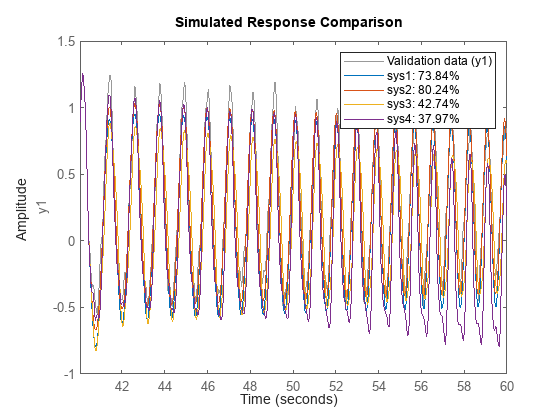
The compare plots indicates sys2 as the best model. Note that the regressors used in this example were chosen arbitrarily, mainly to show the different way of creating regressors and estimating models. Better results can be obtained by picking regressors more judiciously.
MIMO Example: Modeling a Motorized Camera
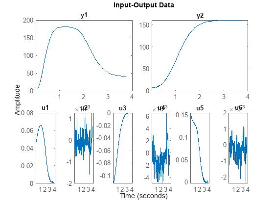
The file motorizedcamera.mat contains one data set with 188 data samples, collected from a motorized camera at a sampling rate of 0.02 second. The input vector u(t) is composed of 6 variables: the 3 translation velocity components in the orthogonal X-Y-Z coordinate system fixed to the camera [m/s], and the 3 rotation velocity components around the X-Y-Z axis [rad/s]. The output vector y(t) contains 2 variables: the position (in pixel) of a point which is the image taken by the camera of a fixed point in the 3D space. We create an IDDATA object z to hold the loaded data:
load motorizedcamera
z = iddata(y, u, 0.02, 'Name', 'Motorized Camera', 'TimeUnit', 's');
stackedplot(iddata2timetable(z))
Using different types of regressors in the MIMO case is not very different from the SISO case. All the regressors are used in the dynamics for all the outputs of the system. The RegressorUsage property may be used to assign specific regressors to be used for specific outputs.
nanbnk = [ones(2,2), 2*ones(2,6), ones(2,6)];
sysMIMO = idnlarx(z.OutputName, z.InputName, nanbnk, idLinear);
C = customRegressor({'u5','u6'},{1 1},@(x,y)x.*y);
P1 = polynomialRegressor('u1',1,2);
P2 = polynomialRegressor('y2',1,3);
sysMIMO.Regressors = [sysMIMO.Regressors; C; P1; P2];
getreg(sysMIMO)
ans = 17×1 cell
{'y1(t-1)' }
{'y2(t-1)' }
{'u1(t-1)' }
{'u1(t-2)' }
{'u2(t-1)' }
{'u2(t-2)' }
{'u3(t-1)' }
{'u3(t-2)' }
{'u4(t-1)' }
{'u4(t-2)' }
{'u5(t-1)' }
{'u5(t-2)' }
{'u6(t-1)' }
{'u6(t-2)' }
{'u1(t-1)^2' }
{'y2(t-1)^3' }
{'u5(t-1).*u6(t-1)'}
sysMIMO = nlarx(z, sysMIMO)
sysMIMO =

Nonlinear ARX model with 2 outputs and 6 inputs
  Inputs: u1, u2, u3, u4, u5, u6
  Outputs: y1, y2

Regressors:
  1. Linear regressors in variables y1, y2, u1, u2, u3, u4, u5, u6
  2. Order 2 regressors in variables u1
  3. Order 3 regressors in variables y2
  4. Custom regressor: u5(t-1).*u6(t-1)
  List of all regressors

Output functions:
  Output 1:  Linear with offset
  Output 2:  Linear with offset

Sample time: 0.02 seconds

Status:
Estimated using NLARX on time domain data "Motorized Camera".
Fit to estimation data: [99.05;98.85]% (prediction focus)
FPE: 0.2067, MSE: 0.7496

Model Properties
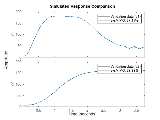
Compare model response to estimation data.
compare(z,sysMIMO)
Analyze model residuals for their auto-correlation (whiteness test) and cross-correlation to the input signal (correlation test).
fig = figure;
fig.Position(3) = 2*fig.Position(3);
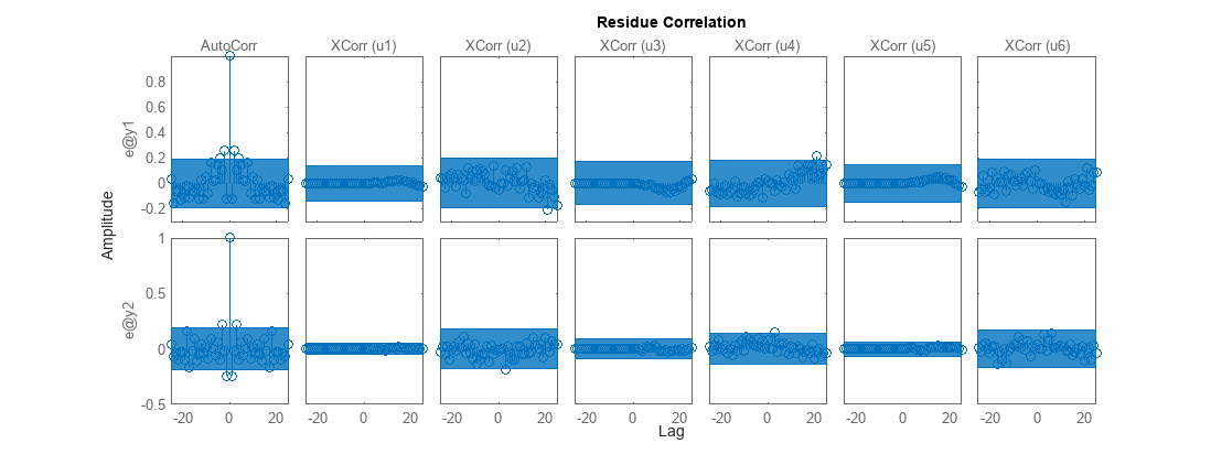
resid(z,sysMIMO)
