What Is Residual Analysis?
Residuals are differences between the one-step-ahead predicted output from the model and the measured output from the validation data set. Thus, residuals represent the portion of the validation data not explained by the model.
Residual analysis consists of two tests: the whiteness test and the independence test.
According to the whiteness test criteria, a good model has the residual autocorrelation function inside the confidence interval of the corresponding estimates, indicating that the residuals are uncorrelated.
According to the independence test criteria, a good model has residuals uncorrelated with past inputs. Evidence of correlation indicates that the model does not describe how part of the output relates to the corresponding input. For example, a peak outside the confidence interval for lag k means that the output y(t) that originates from the input u(t-k) is not properly described by the model.
Your model should pass both the whiteness and the independence tests, except in the following cases:
For output-error (OE) models and when using instrumental-variable (IV) methods, make sure that your model shows independence of
eandu, and pay less attention to the results of the whiteness ofe.In this case, the modeling focus is on the dynamics G and not the disturbance properties H.
Correlation between residuals and input for negative lags, is not necessarily an indication of an inaccurate model.
When current residuals at time t affect future input values, there might be feedback in your system. In the case of feedback, concentrate on the positive lags in the cross-correlation plot during model validation.
Supported Model Types
You can validate parametric linear and nonlinear models by checking the behavior of the model residuals. For a description of residual analysis, see What Residual Plots Show for Different Data Domains.
Note
Residual analysis plots are not available for frequency response (FRD) models. For time-series models, you can only generate model-output plots for parametric models using time-domain time-series (no input) measured data.
What Residual Plots Show for Different Data Domains
Residual analysis plots show different information depending on whether you use time-domain or frequency-domain input-output validation data.
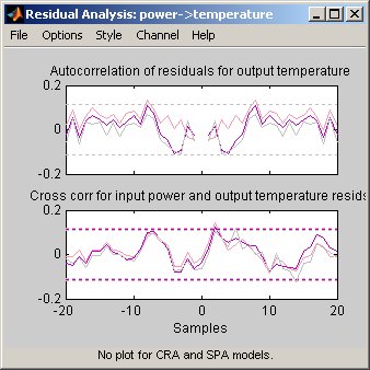
For time-domain validation data, the plot shows the following two axes:
Autocorrelation function of the residuals for each output
Cross-correlation between the input and the residuals for each input-output pair
Note
For time-series models, the residual analysis plot does not provide any input-residual correlation plots.
For frequency-domain validation data, the plot shows the following two axes:
Estimated power spectrum of the residuals for each output
Transfer-function amplitude from the input to the residuals for each input-output pair
For linear models, you can estimate a model using time-domain data, and then validate the model using frequency domain data. For nonlinear models, the System Identification Toolbox™ product supports only time-domain data.
The following figure shows a sample Residual Analysis plot, created in the System Identification app.
Displaying the Confidence Interval
The confidence interval corresponds to the range of residual values with a specific probability of being statistically insignificant for the system. The toolbox uses the estimated uncertainty in the model parameters to calculate confidence intervals and assumes the estimates have a Gaussian distribution.
For example, for a 95% confidence interval, the region around zero represents the range of residual values that have a 95% probability of being statistically insignificant. You can specify the confidence interval as a probability (between 0 and 1) or as the number of standard deviations of a Gaussian distribution. For example, a probability of 0.99 (99%) corresponds to 2.58 standard deviations.
You can display a confidence interval on the plot in the app to gain insight into the quality of the model. To learn how to show or hide confidence interval, see the description of the plot settings in How to Plot Residuals in the App.
Note
If you are working in the System Identification app, you can
specify a custom confidence interval. If you are using the resid command, the confidence interval
is fixed at 99%.