Compare Air Resistance Models for Projectile Motion

Since R2023b

This example shows how to use Experiment Manager to compare the effects of air resistance on the trajectory of a projectile assuming one of these models:

• No air resistance — The motion of the projectile depends only on gravity.

• Stokes drag — Air resistance is proportional to velocity.

• Newton drag — Air resistance is proportional to the square of velocity.

In this experiment, you observe the differences in trajectory shape, height, and range, and determine the launch angle that produces the longest projectile range for each air resistance model.

Open Experiment

First, open the example. Experiment Manager loads a project with a preconfigured experiment that you can inspect and run. To open the experiment, in the Experiment Browser pane, double-click AirResistanceExperiment.

The experiment consists of a description, a table of parameters, and an experiment function. For more information, see Configure General-Purpose Experiment.

The Description field contains a textual description of the experiment. For this example, the description is:

Simulate projectile motion defined by angle Theta, coefficient of friction Mu, and one of these models:
* None - no air resistance
* Stokes - air resistance is proportional to velocity
* Newton - air resistance is proportional to the square of velocity

The Parameters section specifies the parameter values to use for the experiment. Experiment Manager runs multiple trials of your experiment using a different combination of parameters for each trial. In this example, the parameters Model, Theta, and Mu specify the air resistance model, the launch angle, and the coefficient of friction, respectively. Model is a string with the values "None", "Stokes", and "Newton", Theta takes five values between 15 and 75 degrees, and Mu has a constant value of 0.02.

The Experiment Function section specifies the function AirResistanceFunction, which defines the procedure for the experiment. To open this function in MATLAB® Editor, click Edit. The code for the function also appears in Experiment Function. The input to the experiment function is a structure called params with fields from the parameter table. The function uses dot notation to extract the parameter values from this structure and to set up the initial conditions and differential equations for the projectile motion problem.

theta = params.Theta;
mu = params.Mu;
g = 9.81;
vInitial = 300;
 
tInitial = 0;
tFinal = 2*vInitial*sind(theta)/g + 1;
 
yInitial = [0; 0; vInitial*cosd(theta); vInitial*sind(theta)];
 
switch params.Model
    case "None"
        dydt = @(t,y) [y(3); y(4); 0; -g];
    case "Stokes"
        dydt = @(t,y) [y(3); y(4); -mu*y(3); -g-mu*y(4)];
    case "Newton"
        dydt = @(t,y) [y(3); y(4); -mu*y(3)*sqrt(y(3)^2+y(4)^2); ...
            -g-mu*y(4)*sqrt(y(3)^2+y(4)^2)];
    otherwise
        error("Invalid air resistance model")
end

Next, the experiment function calls ode45 to solve the differential equations and to compute the maximum height and range reached by the projectile, as well as the time it takes the projectile to reach these points in the trajectory. The event functions endOfAscent and endOfDescent stop the integration when the projectile reaches the highest point in the trajectory and when it returns to a height of zero.

options = odeset('Events',@endOfAscent);
[~,yout,te,ye,~] = ode45(dydt,[tInitial tFinal],yInitial,options);
tMaxHeight = te;
maxHeight = ye(2);
 
tInitial = te;
yInitial = ye';
options = odeset('Events',@endOfDescent);
[~,y,te,ye,~] = ode45(dydt,[tInitial tFinal],yInitial,options);
yout = [yout; y(2:end,:)];
tMaxRange = te;
maxRange = ye(1);

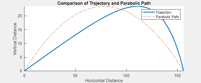
Finally, the experiment function plots the predicted trajectory of the projectile and a parabolic path with the same height and range. When you run the experiment, Experiment Manager adds a button to the Review Results gallery in the toolstrip so you can display the figure. The Name property of the figure specifies the name of the button in the toolstrip.

figure(Name="Projectile Trajectory")
hold on
plot(yout(:,1),yout(:,2),LineWidth=2)
X = maxRange*(0:0.05:1);
Y = 4*maxHeight*X.*(maxRange-X)/maxRange^2;
plot(X,Y,"-.")
title("Comparison of Trajectory and Parabolic Path")
xlabel("Horizontal Distance")
ylabel("Vertical Distance")
legend("Trajectory","Parabolic Path")
axis tight
hold off

Run Experiment

On the Experiment Manager toolstrip, click Run. Experiment Manager runs the experiment function 15 times, each time using a different combination of parameter values. A table of results displays the output values for each trial.

Evaluate Results

The results table shows that the height and range of the predicted trajectory decrease as air resistance increases. To visualize the effects of air resistance on the shape of the trajectory, select a trial. Then, on the Experiment Manager toolstrip, under Review Results, click Projectile Trajectory. When there is no air resistance, the trajectory of the projectile is a parabola.

The Stokes drag model offsets the trajectory slightly to the right of a parabolic path with the same height and range.

In contrast, the trajectory under the Newton drag model is shifted significantly to the right of a parabolic path.

To investigate how the launch angle affects the maximum range of the projectile under each model, sort the results table by maximum range and by model:

1. Point to the header of the maxRange column.

2. Click the triangle icon.

3. Select Sort in Descending Order.

4. Repeat the previous steps for the Model column, but select Sort in Ascending Order.

When there is no air resistance, the maximum range occurs at a launch angle of 45 degrees. For the Newton drag model, the maximum range occurs between 15 and 30 degrees, and for the Stokes drag model, the maximum range occurs between 30 and 45 degrees.

Rerun Experiment

To identify the launch angle that maximizes the range of the projectile with greater precision, change the parameter values and rerun the experiment:

1. Return to the experiment definition tab.

2. In the parameter table, change the value of the parameter Model to "Newton".

3. Change the value of the parameter Theta to 15:30.

4. Run the experiment using the new parameter values.

Experiment Manager runs the experiment function 16 times, each time using the Newton drag model and a different launch angle between 15 and 30 degrees.

The results show that the maximum range for the Newton drag model occurs at approximately 24 degrees. A similar approach shows that the maximum range for the Stokes drag model occurs at approximately 39 degrees.

Close Experiment

In the Experiment Browser pane, right-click ProjectileMotionProject and select Close Project. Experiment Manager closes the experiment and results contained in the project.

Experiment Function

This function extracts the values in the parameter table and sets up the initial conditions and differential equations for the projectile motion problem. The function calls ode45 to solve the differential equations and to compute the maximum height and range reached by the projectile, as well as the time it takes the projectile to reach these points in the trajectory. Then, the function plots the trajectory of the projectile and a parabolic path with the same height and range.

function [maxHeight,maxRange,tMaxHeight,tMaxRange] = AirResistanceFunction(params)

theta = params.Theta;
mu = params.Mu;
g = 9.81;
vInitial = 300;
 
tInitial = 0;
tFinal = 2*vInitial*sind(theta)/g + 1;
 
yInitial = [0; 0; vInitial*cosd(theta); vInitial*sind(theta)];
 
switch params.Model
    case "None"
        dydt = @(t,y) [y(3); y(4); 0; -g];
    case "Stokes"
        dydt = @(t,y) [y(3); y(4); -mu*y(3); -g-mu*y(4)];
    case "Newton"
        dydt = @(t,y) [y(3); y(4); -mu*y(3)*sqrt(y(3)^2+y(4)^2); ...
            -g-mu*y(4)*sqrt(y(3)^2+y(4)^2)];
    otherwise
        error("Invalid air resistance model")
end
 
options = odeset('Events',@endOfAscent);
[~,yout,te,ye,~] = ode45(dydt,[tInitial tFinal],yInitial,options);
tMaxHeight = te;
maxHeight = ye(2);
 
tInitial = te;
yInitial = ye';
options = odeset('Events',@endOfDescent);
[~,y,te,ye,~] = ode45(dydt,[tInitial tFinal],yInitial,options);
yout = [yout; y(2:end,:)];
tMaxRange = te;
maxRange = ye(1);
 
figure(Name="Projectile Trajectory")
hold on
plot(yout(:,1),yout(:,2),LineWidth=2)
X = maxRange*(0:0.05:1);
Y = 4*maxHeight*X.*(maxRange-X)/maxRange^2;
plot(X,Y,"-.")
title("Comparison of Trajectory and Parabolic Path")
xlabel("Horizontal Distance")
ylabel("Vertical Distance")
legend("Trajectory","Parabolic Path")
axis tight
hold off
 
end

Helper Functions

This event function stops the integration when the projectile reaches the highest point in the trajectory.

function [value,isterminal,direction] = endOfAscent(~,y)
value = y(4);
isterminal = 1;
direction = 0;
end

This event function stops the integration when the projectile returns to a height of zero.

function [value,isterminal,direction] = endOfDescent(~,y)
value = y(2);
isterminal = 1;
direction = 0;
end