Solve PDE and Compute Partial Derivatives
This example shows how to solve a transistor partial differential equation (PDE) and use the results to obtain partial derivatives that are part of solving a larger problem.
Consider the PDE
This equation arises in transistor theory [1], and is a function describing the concentration of excess charge carriers (or holes) in the base of a PNP transistor. and are physical constants. The equation holds on the interval for times .
The initial condition includes a constant and is given by
The problem has boundary conditions given by
For fixed , the solution to the equation describes the collapse of excess charge as . This collapse produces a current, called the emitter discharge current, which has another constant :
The equation is valid for due to the inconsistency in the boundary values at for and . Since the PDE has a closed-form series solution for , you can calculate the emitter discharge current analytically as well as numerically, and compare the results.
To solve this problem in MATLAB®, you need to code the PDE equation, initial conditions, and boundary conditions, then select a suitable solution mesh before calling the solver pdepe. You either can include the required functions as local functions at the end of a file (as done here), or save them as separate, named files in a directory on the MATLAB path.
Define Physical Constants
To keep track of the physical constants, create a structure array with fields for each one. When you later define functions for the equations, the initial condition, and the boundary conditions, you can pass in this structure as an extra argument so that the functions have access to the constants.
C.L = 1;
C.D = 0.1;
C.eta = 10;
C.K = 1;
C.Ip = 1;
Code Equation
Before you can code the equation, you need to make sure that it is in the form that the pdepe solver expects:
In this form, the PDE is
So the values of the coefficients in the equation are
(Cartesian coordinates with no angular symmetry)
Now you can create a function to code the equation. The function should have the signature [c,f,s] = transistorPDE(x,t,u,dudx,C):
xis the independent spatial variable.tis the independent time variable.uis the dependent variable being differentiated with respect toxandt.dudxis the partial spatial derivative .Cis an extra input containing the physical constants.The outputs
c,f, andscorrespond to coefficients in the standard PDE equation form expected bypdepe.
As a result, the equation in this example can be represented by the function:
function [c,f,s] = transistorPDE(x,t,u,dudx,C)
D = C.D;
eta = C.eta;
L = C.L;

c = 1;
f = D*dudx;
s = -(D*eta/L)*dudx;
end
(Note: All functions are included as local functions at the end of the example.)
Code Initial Condition
Next, write a function that returns the initial condition. The initial condition is applied at the first time value, and provides the value of for any value of . Use the function signature u0 = transistorIC(x,C) to write the function.
The initial condition is
The corresponding function is
function u0 = transistorIC(x,C)
K = C.K;
L = C.L;
D = C.D;
eta = C.eta;

u0 = (K*L/D)*(1 - exp(-eta*(1 - x/L)))/eta;
end
Code Boundary Conditions
Now, write a function that evaluates the boundary conditions . For problems posed on the interval , the boundary conditions apply for all and either or . The standard form for the boundary conditions expected by the solver is
Written in this form, the boundary conditions for this problem are
- For , the equation is The coefficients are:
- Likewise for , the equation is The coefficients are:
The boundary function should use the function signature [pl,ql,pr,qr] = transistorBC(xl,ul,xr,ur,t):
The inputs x
land ulcorrespond to and for the left boundary.The inputs
xrandurcorrespond to and for the right boundary.tis the independent time variable.The outputs
plandqlcorrespond to and for the left boundary ( for this problem).The outputs
prandqrcorrespond to and for the right boundary ( for this problem).
The boundary conditions in this example are represented by the function:
function [pl,ql,pr,qr] = transistorBC(xl,ul,xr,ur,t)
pl = ul;
ql = 0;
pr = ur;
qr = 0;
end
Select Solution Mesh
The solution mesh defines the values of and where the solution is evaluated by the solver. Since the solution to this problem changes rapidly, use a relatively fine mesh of 50 spatial points in the interval and 50 time points in the interval .
x = linspace(0,C.L,50);
t = linspace(0,1,50);
Solve Equation
Finally, solve the equation using the symmetry , the PDE equation, the initial condition, the boundary conditions, and the meshes for and . Since pdepe expects the PDE function to use four inputs and the initial condition function to use one input, create function handles that pass in the structure of physical constants as an extra input.
m = 0;
eqn = @(x,t,u,dudx) transistorPDE(x,t,u,dudx,C);
ic = @(x) transistorIC(x,C);
sol = pdepe(m,eqn,ic,@transistorBC,x,t);
pdepe returns the solution in a 3-D array sol, where sol(i,j,k) approximates the kth component of the solution evaluated at t(i) and x(j). For this problem u has only one component, but in general you can extract the kth solution component with the command u = sol(:,:,k).
u = sol(:,:,1);
Plot Solution
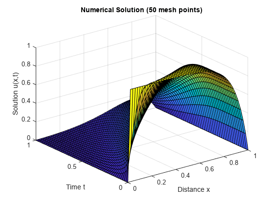
Create a surface plot of the solution plotted at the selected mesh points for and .
surf(x,t,u)
title('Numerical Solution (50 mesh points)')
xlabel('Distance x')
ylabel('Time t')
zlabel('Solution u(x,t)')
Now, plot just and to get a side view of the contours in the surface plot.
plot(x,u)
xlabel('Distance x')
ylabel('Solution u(x,t)')
title('Solution profiles at several times')

Compute Emitter Discharge Current
Using a series solution for , the emitter discharge current can be expressed as the infinite series [1]:
Write a function to calculate the analytic solution for using 40 terms in the series. The only variable is time, but specify a second input to the function for the structure of constants.
function It = serex3(t,C) % Approximate I(t) by series expansion.
Ip = C.Ip;
eta = C.eta;
D = C.D;
L = C.L;

It = 0;
for n = 1:40 % Use 40 terms
  m = (n*pi)^2 + 0.25*eta^2;
  It = It + ((n*pi)^2 / m)* exp(-(D/L^2)*m*t);
end
It = 2*Ip*((1 - exp(-eta))/eta)*It;
end
Using the numeric solution for as computed by pdepe, you can also calculate the numeric approximation for at with
Calculate the analytic and numeric solutions for and plot the results. Use pdeval to compute the value of at .
nt = length(t);
I = zeros(1,nt);
seriesI = zeros(1,nt);
iok = 2:nt;
for j = iok
   % At time t(j), compute du/dx at x = 0.
   [~,I(j)] = pdeval(m,x,u(j,:),0);
   seriesI(j) = serex3(t(j),C);
end
% Numeric solution has form I(t) = (I_p*D/K)*du(0,t)/dx
I = (C.Ip*C.D/C.K)*I;

plot(t(iok),I(iok),'o',t(iok),seriesI(iok))
legend('From PDEPE + PDEVAL','From series')
title('Emitter discharge current I(t)')
xlabel('Time t')
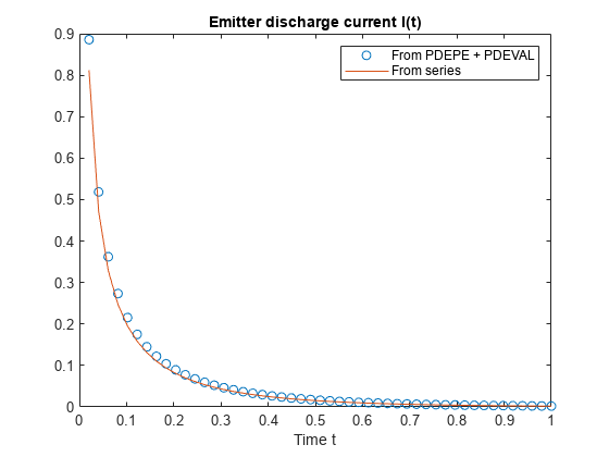
The results match reasonably well. You can further improve the numeric result from pdepe by using a finer solution mesh.
Local Functions
Listed here are the local helper functions that the PDE solver pdepe calls to calculate the solution. Alternatively, you can save these functions as their own files in a directory on the MATLAB path.
function [c,f,s] = transistorPDE(x,t,u,dudx,C) % Equation to solve
D = C.D;
eta = C.eta;
L = C.L;

c = 1;
f = D*dudx;
s = -(D*eta/L)*dudx;
end
% ----------------------------------------------------
function u0 = transistorIC(x,C) % Initial condition
K = C.K;
L = C.L;
D = C.D;
eta = C.eta;

u0 = (K*L/D)*(1 - exp(-eta*(1 - x/L)))/eta;
end
% ----------------------------------------------------
function [pl,ql,pr,qr] = transistorBC(xl,ul,xr,ur,t) % Boundary conditions
pl = ul;
ql = 0;
pr = ur;
qr = 0;
end
% ----------------------------------------------------
function It = serex3(t,C) % Approximate I(t) by series expansion.
Ip = C.Ip;
eta = C.eta;
D = C.D;
L = C.L;

It = 0;
for n = 1:40 % Use 40 terms
  m = (n*pi)^2 + 0.25*eta^2;
  It = It + ((n*pi)^2 / m)* exp(-(D/L^2)*m*t);
end
It = 2*Ip*((1 - exp(-eta))/eta)*It;
end
% ----------------------------------------------------
References
[1] Zachmanoglou, E.C. and D.L. Thoe. Introduction to Partial Differential Equations with Applications. Dover, New York, 1986.