Verify BVP Consistency Using Continuation
This example shows how to use continuation to gradually extend a BVP solution to larger intervals.
Falkner-Skan boundary value problems [1] arise from similarity solutions of a viscous, incompressible, laminar flow over a flat plate. An example equation is
.
The problem is posed on the infinite interval with , subject to the boundary conditions
,
,
.
The BVP cannot be solved on the infinite interval, and it is impractical to solve the BVP in a very large finite interval. Instead, this example solves a sequence of problems posed on the smaller interval to verify that the solution has consistent behavior as . This practice of breaking the problem up into simpler problems, with the solution of each problem feeding back in as the initial guess for the next problem, is called continuation.
To solve this system of equations in MATLAB®, you need to code the equations, boundary conditions, and options before calling the boundary value problem solver bvp4c. You either can include the required functions as local functions at the end of a file (as done here), or save them as separate, named files in a directory on the MATLAB path.
Code Equation
Create a function to code the equations. This function should have the signature dfdx = fsode(x,f), where:
x is the independent variable.
f is the dependent variable.
You can rewrite the third-order equation as a system of first-order equations using the substitutions , , and . The equations become
,
,
.
The corresponding function is
function dfdeta = fsode(x,f)
b = 0.5;
dfdeta = [ f(2)
           f(3)
          -f(1)*f(3) - b*(1 - f(2)^2) ];
end
Note: All functions are included as local functions at the end of the example.
Code Boundary Conditions
Now, write a function that returns the residual value of the boundary conditions at the boundary points. This function should have the signature res = fsbc(f0,finf), where:
f0is the value of the boundary condition at the beginning of the interval.finfis the value of the boundary condition at the end of the interval.
To calculate the residual values, you need to put the boundary conditions in the form . In this form, the boundary conditions are
,
,
.
The corresponding function is
function res = fsbc(f0,finf)
res = [f0(1)
       f0(2)
       finf(2) - 1];
end
Create Initial Guess
Lastly, you must provide an initial guess for the solution. A crude mesh of five points and a constant guess that satisfies the boundary conditions are good enough to get convergence on the interval . The variable infinity denotes the right-hand limit of the interval of integration. As the value of infinity increases on subsequent iterations from 3 to its maximum value of 6, the solution from each previous iteration acts as the initial guess for the next iteration.
infinity = 3;
maxinfinity = 6;
solinit = bvpinit(linspace(0,infinity,5),[0 0 1]);
Solve Equation and Plot Solutions
Solve the problem in the initial interval . Plot the solution, and compare the value of to the analytic value [1].
sol = bvp4c(@fsode,@fsbc,solinit);
x = sol.x;
f = sol.y;
plot(x,f(2,:),x(end),f(2,end),'o');
axis([0 maxinfinity 0 1.4]);
title('Falkner-Skan Equation, Positive Wall Shear, \beta = 0.5.')
xlabel('x')
ylabel('df/dx')
hold on
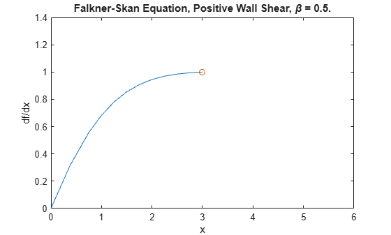
fprintf('Cebeci & Keller report that f''''(0) = 0.92768.\n')Cebeci & Keller report that f''(0) = 0.92768.
fprintf('Value computed using infinity = %g is %7.5f.\n', ...
         infinity,f(3,1))
Value computed using infinity = 3 is 0.92915.
Now, solve the problem on progressively larger intervals by increasing the value of infinity for each iteration. The bvpinit function extrapolates each solution to the new interval to act as the initial guess for the next value of infinity. Each iteration prints the calculated value of and superimposes the plot of the solution over the previous solutions. When infinity = 6, the consistent behavior of the solution becomes evident and the value of is very close to the predicted value.
for Bnew = infinity+1:maxinfinity
  solinit = bvpinit(sol,[0 Bnew]); % Extend solution to new interval
  sol = bvp4c(@fsode,@fsbc,solinit);
  x = sol.x;
  f = sol.y;

  fprintf('Value computed using infinity = %g is %7.5f.\n', ...
           Bnew,f(3,1))
  plot(x,f(2,:),x(end),f(2,end),'o');
  drawnow
end
Value computed using infinity = 4 is 0.92774.
Value computed using infinity = 5 is 0.92770.
Value computed using infinity = 6 is 0.92770.
hold off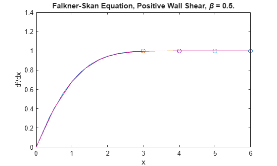
Local Functions
Listed here are the local helper functions that the BVP solver bvp4c calls to calculate the solution. Alternatively, you can save these functions as their own files in a directory on the MATLAB path.
function dfdeta = fsode(x,f) % equation being solved
dfdeta = [ f(2)
           f(3)
          -f(1)*f(3) - 0.5*(1 - f(2)^2) ];
end
%-------------------------------------------
function res = fsbc(f0,finf) % boundary conditions
res = [f0(1)
       f0(2)
       finf(2) - 1];
end
%-------------------------------------------
References
[1] Cebeci, T. and H. B. Keller. "Shooting and Parallel Shooting Methods for Solving the Falkner-Skan Boundary-layer Equation*.*" J. Comp. Phys., Vol. 7, 1971, pp. 289-300.