quad2d

Numerically evaluate double integral — tiled method

Syntax

q = quad2d(fun,a,b,c,d)

q = quad2d(fun,a,b,c,d,Name,Value)

[q,E] = quad2d(___)

Description

q = quad2d(fun,a,b,c,d) approximates the integral of fun(x,y) over the planar region $$a\le x\le b$$ and $$c(x)\le y\le d(x)$$. The bounds c and d can each be scalars or function handles.

q = quad2d(fun,a,b,c,d,Name,Value) specifies additional options with one or more Name,Value pair arguments. For example, you can specify 'AbsTol' and 'RelTol' to adjust the error thresholds that the algorithm must satisfy.

[q,E] = quad2d(___) also returns an approximate upper bound on the absolute error, E = | q - I |, where I is the exact value of the integral.

Examples

Evaluate Double Integral

Integrate

$$y\sin (x)+x\cos (y)$$

over $$-\pi \le x\le 2\pi$$ and $$0\le y\le \pi$$.

fun = @(x,y) y.*sin(x)+x.*cos(y);
Q = quad2d(fun,pi,2*pi,0,pi)

Q = 
-9.8696

Compare the result to the true value of the integral, $$-{\pi }^2$$.

-pi^2

ans = 
-9.8696

Integrand with Singularity on Integration Boundary

Integrate the function

$${\left[{(x+y)}^{1/2}{(1+x+y)}^2\right]}^{-1}$$

over the region $$0\le x\le 1$$ and $$0\le y\le 1-x$$. This integrand is infinite at the origin (0,0), which lies on the boundary of the integration region.

fun = @(x,y) 1./(sqrt(x + y) .* (1 + x + y).^2 );
ymax = @(x) 1 - x;
Q = quad2d(fun,0,1,0,ymax)

Q = 
0.2854

The true value of the integral is $$\pi /4-1/2$$.

pi/4 - 0.5

ans = 
0.2854

Limitations of quad2d

quad2d begins by mapping the region of integration to a rectangle. Consequently, it may have trouble integrating over a region that does not have four sides or has a side that cannot be mapped smoothly to a straight line. If the integration is unsuccessful, some helpful tactics are leaving Singular set to its default value of true, changing between Cartesian and polar coordinates, or breaking the region of integration into pieces and adding the results of integration over the pieces.

For instance:

fun = @(x,y)abs(x.^2 + y.^2 - 0.25);
c = @(x)-sqrt(1 - x.^2);
d = @(x)sqrt(1 - x.^2);
quad2d(fun,-1,1,c,d,'AbsTol',1e-8,...
    'FailurePlot',true,'Singular',false);

Warning: Reached the maximum number of function evaluations (2000). The result fails the global error test.

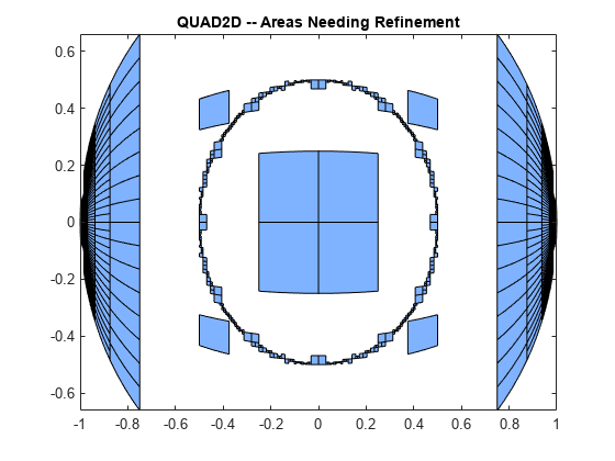
The failure plot shows two areas of difficulty, near the points (-1,0) and (1,0) and near the circle $$x^2+y^2=0.25$$.

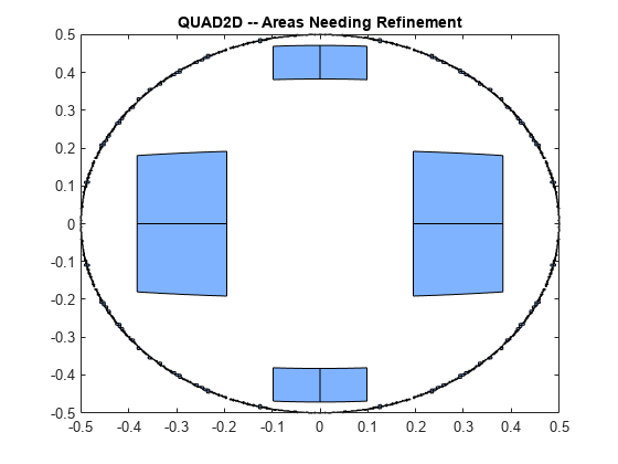
Changing the value of Singular to true will cope with the geometric singularities at (-1,0) and (1,0). The larger shaded areas may need refinement but are probably not areas of difficulty.

Q = quad2d(fun,-1,1,c,d,'AbsTol',1e-8, ... 
     'FailurePlot',true,'Singular',true);

Warning: Reached the maximum number of function evaluations (2000). The result passes the global error test.

From here you can take advantage of symmetry:

Q = 4*quad2d(fun,0,1,0,d,'Abstol',1e-8,...
     'Singular',true,'FailurePlot',true)

Q = 
0.9817

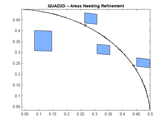
However, the code is still working very hard near the singularity. It may not be able to provide higher accuracy:

Q = 4*quad2d(fun,0,1,0,d,'Abstol',1e-10,...
     'Singular',true,'FailurePlot',true);

Warning: Reached the maximum number of function evaluations (2000). The result passes the global error test.

At higher accuracy, a change in coordinates may work better.

polarfun = @(theta,r) fun(r.*cos(theta),r.*sin(theta)).*r;
Q = 4*quad2d(polarfun,0,pi/2,0,1,'AbsTol',1e-10);

It is best to put the singularity on the boundary by splitting the region of integration into two parts:

Q1 = 4*quad2d(polarfun,0,pi/2,0,0.5,'AbsTol',5e-11);
Q2 = 4*quad2d(polarfun,0,pi/2,0.5,1,'AbsTol',5e-11);
Q = Q1 + Q2;

Input Arguments

fun — Function to integrate

function handle

Function to integrate, specified as a function handle. The function Z = fun(X,Y) must accept 2-D matrices X and Y of the same size and return a matrix Z of corresponding values. Therefore, the function must be vectorized (that is, you must use elementwise operators such as .^ instead of matrix operators such as ^). The inputs and outputs of the function must be either single or double precision.

Example: @(x,y) x.^2 - y.^2

Data Types: function_handle

a,b — x limits of integration

scalars

x limits of integration, specified as scalars.

Data Types: single | double
Complex Number Support: Yes

c,d — y limits of integration

scalars | function handles

y limits of integration, specified as scalars or function handles. Each limit can be specified as a scalar or a function handle. If the limits are specified as function handles, then they are functions of the x limit of integration ymin = @x c(x) and ymax = @(x) d(x). The function handles ymin and ymax must accept matrices and return matrices of the same size with the corresponding values. The inputs and outputs of the functions must be either single or double precision.

Data Types: single | double | function_handle
Complex Number Support: Yes

Name-Value Arguments

Specify optional pairs of arguments as Name1=Value1,...,NameN=ValueN, where Name is the argument name and Value is the corresponding value. Name-value arguments must appear after other arguments, but the order of the pairs does not matter.

Before R2021a, use commas to separate each name and value, and enclose Name in quotes.

Example: quad2d(@(x,y) x.*y.^2, 0, 1, 0, 2, 'AbsTol',1e-3) specifies the absolute tolerance for the integration as 1e-3.

AbsTol — Absolute error tolerance

1e-5 (default) | scalar

Absolute error tolerance, specified as the comma-separated pair consisting of 'AbsTol' and a scalar.

quad2d attempts to satisfy ERRBND <= max(AbsTol,RelTol*|Q|). This is absolute error control when |Q| is sufficiently small and relative error control when |Q| is larger. A default tolerance value is used when a tolerance is not specified. The default value of AbsTol is 1e-5. The default value of RelTol is 100*eps(class(Q)). This is also the minimum value of RelTol. Smaller RelTol values are automatically increased to the default value.

RelTol — Relative error tolerance

100*eps(class(q)) (default) | scalar

Relative error tolerance, specified as the comma-separated pair consisting of 'RelTol' and a scalar.

quad2d attempts to satisfy ERRBND <= max(AbsTol,RelTol*|Q|). This is absolute error control when |Q| is sufficiently small and relative error control when |Q| is larger. A default tolerance value is used when a tolerance is not specified. The default value of AbsTol is 1e-5. The default value of RelTol is 100*eps(class(Q)). This is also the minimum value of RelTol. Smaller RelTol values are automatically increased to the default value.

MaxFunEvals — Maximum number of evaluations of fun

2000 (default) | scalar

Maximum number of evaluations of fun, specified as the comma-separated pair consisting of 'MaxFunEvals' and a scalar. Use this option to limit the number of times quad2d evaluates the function fun.

FailurePlot — Toggle to generate failure plot

false or 0 (default) | true or 1

Toggle to generate failure plot, specified as the comma-separated pair consisting of 'FailurePlot' and a numeric or logical 1 (true) or 0 (false). Set FailurePlot to true or 1 to generate a graphical representation of the regions needing further refinement when MaxFunEvals is reached. No plot is generated if the integration succeeds before reaching MaxFunEvals. The failure plot contains (generally) 4-sided regions that are mapped to rectangles internally. Clusters of small regions indicate the areas of difficulty in the integration.

Singular — Toggle to transform boundary singularities

true or 1 (default) | false or 0

Toggle to transform boundary singularities, specified as the comma-separated pair consisting of 'Singular' and a numeric or logical 1 (true) or 0 (false). By default, quad2d employs transformations to weaken boundary singularities for better performance. Set 'Singular' to false or 0 to turn these transformations off, which can provide a performance benefit on some smooth problems.

Output Arguments

q — Calculated integral

scalar

Calculated integral, returned as a scalar.

E — Error bound

scalar

Error bound, returned as a scalar. The error bound provides an upper bound on the error between the calculated integral q and the exact value of the integral I such that E = | q - I |.

References

[1] L.F. Shampine, "MATLAB Program for Quadrature in 2D." Applied Mathematics and Computation. Vol. 202, Issue 1, 2008, pp. 266–274.

Extended Capabilities

C/C++ Code Generation

Generate C and C++ code using MATLAB® Coder™.

Usage notes and limitations:

• Generated code issues a warning if the size of the internal storage arrays is not large enough. If a warning occurs, as a workaround, you can try to divide the region of integration into pieces and sum the integrals over each piece.

Version History

Introduced in R2009a