stairs
Stairstep graph
Syntax
Description
Vector and Matrix Data
stairs( draws a stairstep graph of
the elements in Y)Y.
If
Yis a vector, thenstairsdraws one line.If
Yis a matrix, thenstairsdraws one line per matrix column.
Table Data
stairs(
plots the specified variable from the table against the row indices of the
table. If the table is a timetable, the specified variable is plotted against
the row times of the timetable. To plot one set of y-values,
specify one variable for tbl,yvar)yvar. To plot multiple sets of
y-values, specify multiple variables for
yvar. (since R2022b)
Additional Options
stairs(___,
modifies the stairstep chart using one or more name-value pair arguments. For
example, Name,Value)"Marker","o","MarkerSize",8 specifies 8 point circle
markers.
stairs( plots
into the axes specified by ax,___)ax instead of into the current
axes (gca). The option, ax, can precede
any of the input argument combinations in the previous syntaxes.
h = stairs(___)Stair objects. Use
h to make changes to properties of a specific Stair object after it is created.
Examples
Create a stairstep plot of sine evaluated at 40 equally spaced values between 0 and .
X = linspace(0,4*pi,40);
Y = sin(X);

figure
stairs(Y)

The length of Y automatically determines and generates the x-axis scale.
Create a stairstep plot of two cosine functions evaluated at 50 equally spaced values between 0 and .
X = linspace(0,4*pi,50)';
Y = [0.5*cos(X), 2*cos(X)];

figure
stairs(Y)

The number of rows in Y automatically determines and generates the x-axis scale.
Create a stairstep plot of a sine wave evaluated at equally spaced values between 0 and . Specify the set of x-values for the plot.
X = linspace(0,4*pi,40);
Y = sin(X);

figure
stairs(X,Y)

The entries in Y are plotted against the corresponding entries in X.
Create a stairstep plot of two cosine waves evaluated at equally spaced values between 0 and . Specify the set of x-values for the plot.
X = linspace(0,4*pi,50)';
Y = [0.5*cos(X), 2*cos(X)];

figure
stairs(X,Y)
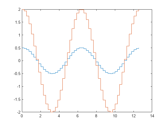
The first vector input, X, determines the x-axis positions for both data series.
Create a stairstep plot of two sine waves evaluated at different values. Specify a unique set of x-values for plotting each data series.
x1 = linspace(0,2*pi)';
x2 = linspace(0,pi)';
X = [x1,x2];
Y = [sin(5*x1),exp(x2).*sin(5*x2)];

figure
stairs(X,Y)
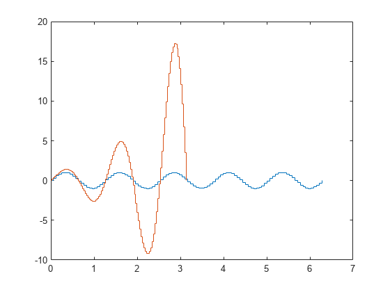
Each column of X is plotted against the corresponding column of Y.
Create a stairstep plot and set the line style to a dot-dashed line, the marker symbol to circles, and the color to red.
X = linspace(0,4*pi,20);
Y = sin(X);

figure
stairs(Y, '-.or')
Create a stairstep plot and set the line width to 2, the marker symbols to diamonds, and the marker face color to cyan using Name,Value pair arguments.
X = linspace(0,4*pi,20);
Y = sin(X);

figure
stairs(Y,'LineWidth',2,'Marker','d','MarkerFaceColor','c')

Since R2022b
A convenient way to plot data from a table is to pass the table to the stairs function and specify the variables to plot.
Read the first 100 rows and 7 columns of weather.csv as a timetable tbl. Then display the first three rows of the table.
tbl = readtimetable("weather.csv","Range",[1 1 101 7]);
head(tbl,3)
            Time            WindDirection    WindSpeed    Humidity    Temperature    RainInchesPerMinute    CumulativeRainfall
    ____________________    _____________    _________    ________    ___________    ___________________    __________________

    25-Oct-2021 00:00:09         46               1          84          49.2                 0                     0
    25-Oct-2021 00:01:09         45             1.6          84          49.2                 0                     0
    25-Oct-2021 00:02:09         36             2.2          84          49.2                 0                     0
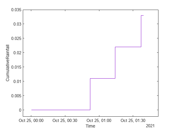
Plot the Time variable on the x-axis and the CumulativeRainfall variable on the y-axis. Then use the axis padded command so that the line and the plot box do not overlap.
Return the Stair object as h. Notice that the axis labels match the variable names.
h = stairs(tbl,"Time","CumulativeRainfall");
axis padded

Change the color of the line to purple by setting the Color property.
h.Color = [0.5 0 0.8];
Since R2022b
Create vectors x, y1, and y2, and use them to create a table. Plot the y1 and y2 variables against the x variable. Use the axis padded command so that the line and the plot box do not overlap.
Add a legend, and notice that the legend labels match the variable names.
x = linspace(0,6,20);
y1 = cos(x);
y2 = sin(x);
tbl = table(x,y1,y2);
stairs(tbl,"x",["y1","y2"]);

% Pad x- and y-axes, and add legend
axis padded
legend

Alternatively, you can omit the x variable and plot the y1 and y2 variables against the row indices of the table.
stairs(tbl,["y1","y2"]);
axis padded
legend

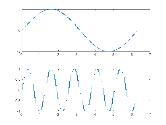
You can display a tiling of plots using the tiledlayout and nexttile functions. Call the tiledlayout function to create a 2-by-1 tiled chart layout. Call the nexttile function to create the axes objects ax1 and ax2. Create separate stairstep plots in the axes by specifying the axes object as the first argument to stairs.
x = linspace(0,2*pi);
y1 = 5*sin(x);
y2 = sin(5*x);
tiledlayout(2,1)

% Top plot
ax1 = nexttile;
stairs(ax1,x,y1)

% Bottom plot
ax2 = nexttile;
stairs(ax2,x,y2)
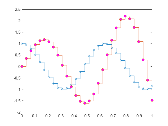
Create a stairstep plot of two data series and return the two stair objects.
X = linspace(0,1,30)';
Y = [cos(10*X), exp(X).*sin(10*X)];
h = stairs(X,Y);

Use small circle markers for the first data series. Use magenta filled circles for the second series. Use dot notation to set properties.
h(1).Marker = 'o';
h(1).MarkerSize = 4;
h(2).Marker = 'o';
h(2).MarkerFaceColor = 'm';
Evaluate two cosine functions at 50 equally spaced values between 0 and and create a stairstep plot using plot.
X = linspace(0,4*pi,50)';
Y = [0.5*cos(X), 2*cos(X)];
[xb,yb] = stairs(X,Y);
stairs returns two matrices of the same size, xb and yb, but no plot.
Use plot to create the stairstep plot with xb and yb.
figure
plot(xb,yb)

Input Arguments
y values, specified as a vector or matrix.
When Y is a vector, stairs creates
one stair object. When Y is a matrix, stairs draws
one line per matrix column and creates a separate stair object for
each column.
Data Types: single | double | int8 | int16 | int32 | int64 | uint8 | uint16 | uint32 | uint64 | categorical | datetime | duration
x values, specified as a vector or matrix.
When Y is a vector, X must be
a vector of the same size. When Y is a matrix, X must
be a matrix of the same size, or a vector whose length equals the
number of rows in Y.
Data Types: single | double | int8 | int16 | int32 | int64 | uint8 | uint16 | uint32 | uint64 | categorical | datetime | duration
Line style, marker, and color, specified as a string scalar or character vector containing symbols. The symbols can appear in any order. You do not need to specify all three characteristics (line style, marker, and color). For example, if you omit the line style and specify the marker, then the plot shows only the marker and no line.
Example: "--or" is a red dashed line with circle markers.
| Line Style | Description | Resulting Line |
|---|---|---|
"-" | Solid line |
|
"--" | Dashed line |
|
":" | Dotted line |
|
"-." | Dash-dotted line |
|
| Marker | Description | Resulting Marker |
|---|---|---|
"o" | Circle |
|
"+" | Plus sign |
|
"*" | Asterisk |
|
"." | Point |
|
"x" | Cross |
|
"_" | Horizontal line |
|
"|" | Vertical line |
|
"square" | Square |
|
"diamond" | Diamond |
|
"^" | Upward-pointing triangle |
|
"v" | Downward-pointing triangle |
|
">" | Right-pointing triangle |
|
"<" | Left-pointing triangle |
|
"pentagram" | Pentagram |
|
"hexagram" | Hexagram |
|
| Color Name | Short Name | RGB Triplet | Appearance |
|---|---|---|---|
"red" | "r" | [1 0 0] |
|
"green" | "g" | [0 1 0] |
|
"blue" | "b" | [0 0 1] |
|
"cyan"
| "c" | [0 1 1] |
|
"magenta" | "m" | [1 0 1] |
|
"yellow" | "y" | [1 1 0] |
|
"black" | "k" | [0 0 0] |
|
"white" | "w" | [1 1 1] |
|
Source table containing the data to plot, specified as a table or timetable.
Table variables containing the y-coordinates, specified using one of the indexing schemes from the table.
| Indexing Scheme | Examples |
|---|---|
Variable names:
|
|
Variable indices:
|
|
Variable type:
|
|
The table variables you specify can contain numeric, categorical,
datetime, or duration values. If xvar and
yvar both specify multiple variables, the number of
variables must be the same.
Example: stairs(tbl,"x",["y1","y2"]) specifies the table
variables named y1 and y2 for the
y-coordinates.
Example: stairs(tbl,"x",2) specifies the second variable
for the y-coordinates.
Example: stairs(tbl,"x",vartype("numeric")) specifies
all numeric variables for the
y-coordinates.
Table variables containing the x-coordinates, specified using one of the indexing schemes from the table.
| Indexing Scheme | Examples |
|---|---|
Variable names:
|
|
Variable indices:
|
|
Variable type:
|
|
The table variables you specify can contain numeric, categorical,
datetime, or duration values. If xvar and
yvar both specify multiple variables, the number of
variables must be the same.
Example: stairs(tbl,["x1","x2"],"y") specifies the table
variables named x1 and x2 for the
x-coordinates.
Example: stairs(tbl,2,"y") specifies the second variable
for the x-coordinates.
Example: stairs(tbl,vartype("numeric"),"y") specifies
all numeric variables for the
x-coordinates.
Axes object. If you do not specify the axes,
then stairs plots into the current axes.
Name-Value Arguments
Specify optional pairs of arguments as
Name1=Value1,...,NameN=ValueN, where Name is
the argument name and Value is the corresponding value.
Name-value arguments must appear after other arguments, but the order of the
pairs does not matter.
Before R2021a, use commas to separate each name and value, and enclose
Name in quotes.
Example: "Marker","s","MarkerFaceColor","red" plots the stairstep graph with
red square markers.
The properties listed here are only a subset. For a complete list, see Stair Properties.
Line style, specified as one of the options listed in this table.
| Line Style | Description | Resulting Line |
|---|---|---|
"-" | Solid line |
|
"--" | Dashed line |
|
":" | Dotted line |
|
"-." | Dash-dotted line |
|
"none" | No line | No line |
Line width, specified as a positive value in points, where 1 point = 1/72 of an inch. If the line has markers, then the line width also affects the marker edges.
The line width cannot be thinner than the width of a pixel. If you set the line width to a value that is less than the width of a pixel on your system, the line is displayed as one pixel wide.
Line color, specified as an RGB triplet, a hexadecimal color code, a color name, or a short name.
For a custom color, specify an RGB triplet or a hexadecimal color code.
An RGB triplet is a three-element row vector whose elements specify the intensities of the red, green, and blue components of the color. The intensities must be in the range
[0,1], for example,[0.4 0.6 0.7].A hexadecimal color code is a string scalar or character vector that starts with a hash symbol (
#) followed by three or six hexadecimal digits, which can range from0toF. The values are not case sensitive. Therefore, the color codes"#FF8800","#ff8800","#F80", and"#f80"are equivalent.
Alternatively, you can specify some common colors by name. This table lists the named color options, the equivalent RGB triplets, and the hexadecimal color codes.
| Color Name | Short Name | RGB Triplet | Hexadecimal Color Code | Appearance |
|---|---|---|---|---|
"red" | "r" | [1 0 0] | "#FF0000" |
|
"green" | "g" | [0 1 0] | "#00FF00" |
|
"blue" | "b" | [0 0 1] | "#0000FF" |
|
"cyan"
| "c" | [0 1 1] | "#00FFFF" |
|
"magenta" | "m" | [1 0 1] | "#FF00FF" |
|
"yellow" | "y" | [1 1 0] | "#FFFF00" |
|
"black" | "k" | [0 0 0] | "#000000" |
|
"white" | "w" | [1 1 1] | "#FFFFFF" |
|
"none" | Not applicable | Not applicable | Not applicable | No color |
This table lists the default color palettes for plots in the light and dark themes.
| Palette | Palette Colors |
|---|---|
Before R2025a: Most plots use these colors by default. |
|
|
|
You can get the RGB triplets and hexadecimal color codes for these palettes using the orderedcolors and rgb2hex functions. For example, get the RGB triplets for the "gem" palette and convert them to hexadecimal color codes.
RGB = orderedcolors("gem");
H = rgb2hex(RGB);
Before R2023b: Get the RGB triplets using RGB =
get(groot,"FactoryAxesColorOrder").
Before R2024a: Get the hexadecimal color codes using H =
compose("#%02X%02X%02X",round(RGB*255)).
Example: "blue"
Example: [0
0 1]
Example: "#0000FF"
Marker symbol, specified as one of the values listed in this table. By default, the object does not display markers. Specifying a marker symbol adds markers at each data point or vertex.
| Marker | Description | Resulting Marker |
|---|---|---|
"o" | Circle |
|
"+" | Plus sign |
|
"*" | Asterisk |
|
"." | Point |
|
"x" | Cross |
|
"_" | Horizontal line |
|
"|" | Vertical line |
|
"square" | Square |
|
"diamond" | Diamond |
|
"^" | Upward-pointing triangle |
|
"v" | Downward-pointing triangle |
|
">" | Right-pointing triangle |
|
"<" | Left-pointing triangle |
|
"pentagram" | Pentagram |
|
"hexagram" | Hexagram |
|
"none" | No markers | Not applicable |
Marker size, specified as a positive value in points, where 1 point = 1/72 of an inch.
Marker outline color, specified as "auto", an RGB triplet, a
hexadecimal color code, a color name, or a short name. The default value of
"auto" uses the same color as the Color
property.
For a custom color, specify an RGB triplet or a hexadecimal color code.
An RGB triplet is a three-element row vector whose elements specify the intensities of the red, green, and blue components of the color. The intensities must be in the range
[0,1], for example,[0.4 0.6 0.7].A hexadecimal color code is a string scalar or character vector that starts with a hash symbol (
#) followed by three or six hexadecimal digits, which can range from0toF. The values are not case sensitive. Therefore, the color codes"#FF8800","#ff8800","#F80", and"#f80"are equivalent.
Alternatively, you can specify some common colors by name. This table lists the named color options, the equivalent RGB triplets, and the hexadecimal color codes.
| Color Name | Short Name | RGB Triplet | Hexadecimal Color Code | Appearance |
|---|---|---|---|---|
"red" | "r" | [1 0 0] | "#FF0000" |
|
"green" | "g" | [0 1 0] | "#00FF00" |
|
"blue" | "b" | [0 0 1] | "#0000FF" |
|
"cyan"
| "c" | [0 1 1] | "#00FFFF" |
|
"magenta" | "m" | [1 0 1] | "#FF00FF" |
|
"yellow" | "y" | [1 1 0] | "#FFFF00" |
|
"black" | "k" | [0 0 0] | "#000000" |
|
"white" | "w" | [1 1 1] | "#FFFFFF" |
|
"none" | Not applicable | Not applicable | Not applicable | No color |
This table lists the default color palettes for plots in the light and dark themes.
| Palette | Palette Colors |
|---|---|
Before R2025a: Most plots use these colors by default. |
|
|
|
You can get the RGB triplets and hexadecimal color codes for these palettes using the orderedcolors and rgb2hex functions. For example, get the RGB triplets for the "gem" palette and convert them to hexadecimal color codes.
RGB = orderedcolors("gem");
H = rgb2hex(RGB);
Before R2023b: Get the RGB triplets using RGB =
get(groot,"FactoryAxesColorOrder").
Before R2024a: Get the hexadecimal color codes using H =
compose("#%02X%02X%02X",round(RGB*255)).
Marker fill color, specified as "auto", an RGB triplet, a hexadecimal
color code, a color name, or a short name. The "auto" option uses the
same color as the Color property of the parent axes. If you specify
"auto" and the axes plot box is invisible, the marker fill color is
the color of the figure.
For a custom color, specify an RGB triplet or a hexadecimal color code.
An RGB triplet is a three-element row vector whose elements specify the intensities of the red, green, and blue components of the color. The intensities must be in the range
[0,1], for example,[0.4 0.6 0.7].A hexadecimal color code is a string scalar or character vector that starts with a hash symbol (
#) followed by three or six hexadecimal digits, which can range from0toF. The values are not case sensitive. Therefore, the color codes"#FF8800","#ff8800","#F80", and"#f80"are equivalent.
Alternatively, you can specify some common colors by name. This table lists the named color options, the equivalent RGB triplets, and the hexadecimal color codes.
| Color Name | Short Name | RGB Triplet | Hexadecimal Color Code | Appearance |
|---|---|---|---|---|
"red" | "r" | [1 0 0] | "#FF0000" |
|
"green" | "g" | [0 1 0] | "#00FF00" |
|
"blue" | "b" | [0 0 1] | "#0000FF" |
|
"cyan"
| "c" | [0 1 1] | "#00FFFF" |
|
"magenta" | "m" | [1 0 1] | "#FF00FF" |
|
"yellow" | "y" | [1 1 0] | "#FFFF00" |
|
"black" | "k" | [0 0 0] | "#000000" |
|
"white" | "w" | [1 1 1] | "#FFFFFF" |
|
"none" | Not applicable | Not applicable | Not applicable | No color |
This table lists the default color palettes for plots in the light and dark themes.
| Palette | Palette Colors |
|---|---|
Before R2025a: Most plots use these colors by default. |
|
|
|
You can get the RGB triplets and hexadecimal color codes for these palettes using the orderedcolors and rgb2hex functions. For example, get the RGB triplets for the "gem" palette and convert them to hexadecimal color codes.
RGB = orderedcolors("gem");
H = rgb2hex(RGB);
Before R2023b: Get the RGB triplets using RGB =
get(groot,"FactoryAxesColorOrder").
Before R2024a: Get the hexadecimal color codes using H =
compose("#%02X%02X%02X",round(RGB*255)).
Output Arguments
Stair objects. These are unique identifiers,
which you can use to query and modify the properties of a specific Stair object
after it is created.
x values for use with plot,
returned as a vector or matrix. xb contains the
appropriate values such that plot(xb,yb) creates
the stairstep graph.
y values for use with plot,
returned as a vector or matrix. yb contains the
appropriate values such that plot(xb,yb) creates
the stairstep graph.
Extended Capabilities
The stairs function
supports GPU array input with these usage notes and limitations:
This function accepts GPU arrays, but does not run on a GPU.
For more information, see Run MATLAB Functions on a GPU (Parallel Computing Toolbox).
The stairs function
supports distributed arrays with these usage notes and limitations:
This function operates on distributed arrays, but executes on the client MATLAB®.
For more information, see Run MATLAB Functions with Distributed Arrays (Parallel Computing Toolbox).
Version History
Introduced before R2006aCreate plots by passing a table to the stairs function
followed by the variables you want to plot. When you specify your data as a table,
the axis labels and the legend (if present) are automatically labeled using the
table variable names.
See Also
Functions
Properties
MATLAB Command
You clicked a link that corresponds to this MATLAB command:
Run the command by entering it in the MATLAB Command Window. Web browsers do not support MATLAB commands.
Sélectionner un site web
Choisissez un site web pour accéder au contenu traduit dans votre langue (lorsqu'il est disponible) et voir les événements et les offres locales. D’après votre position, nous vous recommandons de sélectionner la région suivante : .
Vous pouvez également sélectionner un site web dans la liste suivante :
Comment optimiser les performances du site
Pour optimiser les performances du site, sélectionnez la région Chine (en chinois ou en anglais). Les sites de MathWorks pour les autres pays ne sont pas optimisés pour les visites provenant de votre région.
Amériques
- América Latina (Español)
- Canada (English)
- United States (English)
Europe
- Belgium (English)
- Denmark (English)
- Deutschland (Deutsch)
- España (Español)
- Finland (English)
- France (Français)
- Ireland (English)
- Italia (Italiano)
- Luxembourg (English)
- Netherlands (English)
- Norway (English)
- Österreich (Deutsch)
- Portugal (English)
- Sweden (English)
- Switzerland
- United Kingdom (English)