Design and Evaluate Interleaved ADC
This interleaved ADC model highlights some of the typical impairments introduced by data converters and their effects on a larger system.
Model
In this example, interleave two simple ADCs based on the model Analyzing Simple ADC with Impairments to create the equivalent of one ADC operating at 2X the individual ADC sampling rate.
model = "interleaved_adc";
open_system(model);

Use a two-tone test signal at 203.125 MHz and 218.750 MHz as the input to verify the distortion introduced by the ADC operation. These frequencies were chosen to minimize spectral leakage. They are integer multiples of the Spectrum Analyzer's Resolution Bandwidth (RBW).
set_param(model + "/ADC_1 at 1G SPS", "jitter", "off");
set_param(model + "/ADC_1 at 1G SPS", "nonlinearity", "off");
set_param(model + "/ADC_1 at 1G SPS", "quantization", "off");

set_param(model + "/ADC_2 at 1G SPS", "jitter", "off");
set_param(model + "/ADC_2 at 1G SPS", "nonlinearity", "off");
set_param(model + "/ADC_2 at 1G SPS", "quantization", "off");

set_param(model + "/Offset Delay", "DelayTime", ".5/Fs_adc");
set_param(model + "/Two Tone Sine Wave", "Amplitude", ".5");
set_param(model + "/Two Tone Sine Wave", "Frequency", "2*pi*[203.125, 218.750]*1e6");
set_param(model + "/Input Switch", "sw", "1");

scopeConfig = get_param(model + "/Spectrum Analyzer", "ScopeConfiguration");
scopeConfig.DistortionMeasurements.Type = "intermodulation";
To bypass the impairments, use appropriate switch positions inside the ADC blocks. The ADC behavior is purely ideal. The two ADCs in the top-level model are identical with the exception that the noise generators in each ADC have different seeds to make the noise uncorrelated.
Each ADC operates at 1 GHz rate, set by the MATLAB® variable Fs_adc defined in the initialization callback of this model. The operating rate of the ADCs is indicated by the green signals and blocks in the diagram. The input signal of the second ADC is delayed by an amount equal to half a period of the ADC sampling frequency.
sim(model);

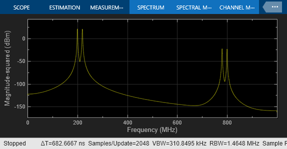
The Spectrum Analyzer shows the unimpaired result of the two-tone test.
Timing Imperfection
The precision of the timing between the individual ADCs is critical. To see the effect of a timing mismatch between the two ADCs, open the Offset Delay block and simply add 10 ps to the delay value.
set_param(model + "/Offset Delay", "DelayTime", ".5/Fs_adc + 10e-12");
The 10 ps error causes a significant degradation of the ADC performance, even though both ADCs are perfectly ideal. To compensate for the performance degradation, some form of drift compensation is necessary. For more information, see Time-Interleaved ADC Error Correction.
sim(model);
The Spectrum Analyzer shows the impact of sample timing mismatch between ADC_1 and ADC_2.
Effect of Aperture Jitter
Remove the fixed offset of 10 ps and enable the aperture jitter impairment in each of the ADC subsystems.
set_param(model + "/Offset Delay", "DelayTime", ".5/Fs_adc");
set_param(model + "/ADC_1 at 1G SPS", "jitter", "on");
set_param(model + "/ADC_2 at 1G SPS", "jitter", "on");
The noise around the two-tone test signal at 200 MHz is expected, as a direct result of the ADC jitter. The additional noise around 800 MHz is the result of interleaving two uncorrelated noise sources.
sim(model);
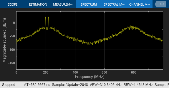
The Spectrum Analyzer shows the effect of aperture jitter on the two-tone test.
Effect of Nonlinearity
Remove the jitter impairment and activate the nonlinearity impairment in both ADCs.
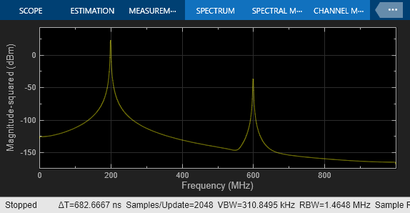
set_param(model + "/ADC_1 at 1G SPS", "jitter", "off");
set_param(model + "/ADC_2 at 1G SPS", "jitter", "off");
set_param(model + "/ADC_1 at 1G SPS", "nonlinearity", "on");
set_param(model + "/ADC_2 at 1G SPS", "nonlinearity", "on");
The spectrum analyzer now shows 3rd order IMD products around two tones and harmonically related spurs around the 600 MHz region.
sim(model);
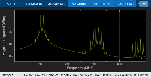
The Spectrum Analyzer shows the impact of nonlinearity in both ADCs.
Even though the ADC nonlinear effects are identical and create exactly the same odd order components, there is actually some cancellation of terms. If just one nonlinearity is enabled, the resulting spectrum is worse than when both ADCs are nonlinear.
set_param(model + "/ADC_2 at 1G SPS", "nonlinearity", "off");
sim(model);
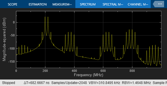
The Spectrum Analyzer shows the impact of nonlinearity in only ADC_1.
Effect of Quantization and Saturation
Remove the linearity impairment and activate the quantization. The quantizer is set to 9 bits, and the signal level is close to the full scale of +/-1, which can be seen in the input Time Scope.
set_param(model + "/ADC_1 at 1G SPS", "nonlinearity", "off");
set_param(model + "/ADC_2 at 1G SPS", "nonlinearity", "off");
set_param(model + "/ADC_1 at 1G SPS", "quantization", "on");
set_param(model + "/ADC_2 at 1G SPS", "quantization", "on");

sim(model);

The Spectrum Analyzer shows the effects of quantization.
Multiply the two tone test signal by a factor of 1.2. The increased amplitude saturates each ADC, producing a clipped waveform and a dirty spectrum.
set_param(model + "/Two Tone Sine Wave", "Amplitude", ".5*1.2");

sim(model);

The Spectrum Analyzer shows the impact of saturating the ADC's input.
ENOB, SFDR, and Other Single Tone Measurements
ADCs are often characterized by their Effective Number of Bits (ENoB), Spurrious-Free Dynamic Range (SFDR), and other similar measurements.
These quantities are derived from a single tone test. To change the ADC's input from the Two Tone Sine Wave source to the Single Tone Sine Wave source and back, double click on the Input Switch. This test uses a single sine wave with a frequency of 200 MHz.
set_param(model + "/Input Switch", "sw", "0");
scopeConfig.DistortionMeasurements.Type = "harmonic";
The ADC AC Measurement block from the Mixed-Signal Blockset™ measures conversion delay, SINAD (the ratio of signal to noise and distortion), SFDR, SNR (Signal to Noise Ratio), ENOB and the ADC's output noise floor.
set_param(model + "/ADC AC Measurement", "Commented", "off");
This block requires a rising edge on its start and ready ports for every conversion that the ADC makes. In this model, these are provided by a 4 GHz pulse generator. To use the ADC AC Measurement block in this model, uncomment the block by right clicking on it and selecting "Uncomment" from the menu. The expected ENOB from a dynamic range of 2 and a least significant bit value (quantization interval) of 2^-8 is 9 bits.
sim(model);
disp(interleaved_adc_output)
           SNR: 51.0747
          SFDR: 60.2803
         SINAD: 51.0394
          ENOB: 8.1859
    NoiseFloor: -292.7286
      MaxDelay: 0
     MeanDelay: 0
      MinDelay: 0
Substitution of ADC Block with System object™
Open the mask dialog of both Flash ADCs in the model "interelaved_flash_adc.slx" and set Simulate using to System object (code generation).
bdclose(model);
model = "interleaved_flash_adc";
load_system(model);

The System Object ADC model is optimized for long simulations, compared to the Simulink block based ADC used earlier in this example. This Flash ADC System Object uses fixed-step discrete sample time and does not support the aperture jitter impairment.
To configure the fixed-step sample rates of the ADCs, set their Sample interval (s) to 1 / (2 * Fs_adc). This is the rate at which the ADC model checks whether or not its inputs have changed. Due to rising edge detection on the conversion start signal, this rate should be at least twice the ADC's sample frequency. Setting Fs_adc to 1e9 and nbits to 9 in the base MATLAB workspace gives this model the same performance as the previous model.
The conversion start signal, specified in the 2x 1 GHz Pulses with 180 deg phase offset block, has the same Sample time of 1 / (2 * Fs_adc). This is the Nyquist rate for that signal. With this Sample time, set the Period to 2 samples, and the Pulse width to 1 sample. Set Phase delay to [0 1] samples to output a vector containing two antiphase conversion start signals. Use the two selector blocks to route the delayed clock signal to the top ADC and the un-delayed clock signal to the Interleaving Switch's initial output comes from its bottom input, input 0, and the second output comes from the top input, input 1.
Set up the ADC AC Measurement block's parameters according to the parameters of the ADC and of the stimulus signal.
open_system(model);

sim(model);

Copyright 2019 The MathWorks, Inc. All rights reserved.