Nonlinear Data-Fitting Using Several Problem-Based Approaches

The general advice for least-squares problem setup is to formulate the problem in a way that allows solve to recognize that the problem has a least-squares form. When you do that, solve internally calls lsqnonlin, which is efficient at solving least-squares problems. See Write Objective Function for Problem-Based Least Squares.

This example shows the efficiency of a least-squares solver by comparing the performance of lsqnonlin with that of fminunc on the same problem. Additionally, the example shows added benefits that you can obtain by explicitly recognizing and handling separately the linear parts of a problem.

Problem Setup

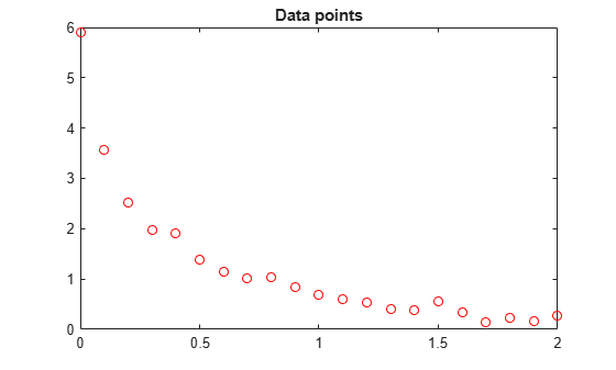
Consider the following data:

Data = ...
  [0.0000    5.8955
   0.1000    3.5639
   0.2000    2.5173
   0.3000    1.9790
   0.4000    1.8990
   0.5000    1.3938
   0.6000    1.1359
   0.7000    1.0096
   0.8000    1.0343
   0.9000    0.8435
   1.0000    0.6856
   1.1000    0.6100
   1.2000    0.5392
   1.3000    0.3946
   1.4000    0.3903
   1.5000    0.5474
   1.6000    0.3459
   1.7000    0.1370
   1.8000    0.2211
   1.9000    0.1704
   2.0000    0.2636];

Plot the data points.

t = Data(:,1);
y = Data(:,2);
plot(t,y,'ro')
title('Data points')

The problem is to fit the function

y = c(1)*exp(-lam(1)*t) + c(2)*exp(-lam(2)*t)

to the data.

Solution Approach Using Default Solver

To begin, define optimization variables corresponding to the equation.

c = optimvar('c',2);
lam = optimvar('lam',2);

Arbitrarily set the initial point x0 as follows: c(1) = 1, c(2) = 1, lam(1) = 1, and lam(2) = 0:

x0.c = [1,1];
x0.lam = [1,0];

Create a function that computes the value of the response at times t when the parameters are c and lam.

diffun = c(1)*exp(-lam(1)*t) + c(2)*exp(-lam(2)*t);

Convert diffun to an optimization expression that sums the squares of the differences between the function and the data y.

diffexpr = sum((diffun - y).^2);

Create an optimization problem having diffexpr as the objective function.

ssqprob = optimproblem('Objective',diffexpr);

Solve the problem using the default solver.

[sol,fval,exitflag,output] = solve(ssqprob,x0)

Solving problem using lsqnonlin.

Local minimum possible.

lsqnonlin stopped because the final change in the sum of squares relative to 
its initial value is less than the value of the function tolerance.

sol = struct with fields:
      c: [2x1 double]
    lam: [2x1 double]

fval = 
0.1477

exitflag = 
    FunctionChangeBelowTolerance

output = struct with fields:
           firstorderopt: 7.8870e-06
              iterations: 6
               funcCount: 7
            cgiterations: 0
               algorithm: 'trust-region-reflective'
                stepsize: 0.0096
                 message: 'Local minimum possible....'
            bestfeasible: []
         constrviolation: []
     objectivederivative: "forward-AD"
    constraintderivative: "closed-form"
                  solver: 'lsqnonlin'

Plot the resulting curve based on the returned solution values sol.c and sol.lam.

resp = evaluate(diffun,sol);
hold on
plot(t,resp)
hold off

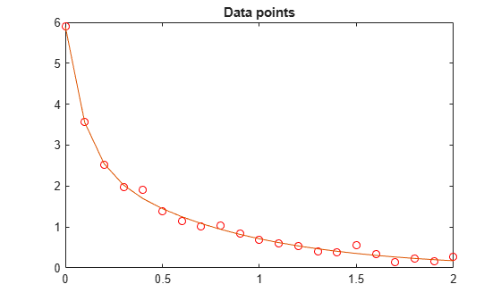
The fit looks to be as good as possible.

Solution Approach Using fminunc

To solve the problem using the fminunc solver, set the 'Solver' option to 'fminunc' when calling solve.

[xunc,fvalunc,exitflagunc,outputunc] = solve(ssqprob,x0,'Solver',"fminunc")

Solving problem using fminunc.

Local minimum found.

Optimization completed because the size of the gradient is less than
the value of the optimality tolerance.

xunc = struct with fields:
      c: [2x1 double]
    lam: [2x1 double]

fvalunc = 
0.1477

exitflagunc = 
    OptimalSolution

outputunc = struct with fields:
             iterations: 30
              funcCount: 37
               stepsize: 0.0017
           lssteplength: 1
          firstorderopt: 2.9454e-05
              algorithm: 'quasi-newton'
                message: 'Local minimum found....'
    objectivederivative: "forward-AD"
                 solver: 'fminunc'

Notice that fminunc found the same solution as lsqcurvefit, but took many more function evaluations to do so. The parameters for fminunc are in the opposite order as those for lsqcurvefit; the larger lam is lam(2), not lam(1). This is not surprising, the order of variables is arbitrary.

fprintf(['There were %d iterations using fminunc,' ...
    ' and %d using lsqcurvefit.\n'], ...
    outputunc.iterations,output.iterations)

There were 30 iterations using fminunc, and 6 using lsqcurvefit.

fprintf(['There were %d function evaluations using fminunc,' ...
    ' and %d using lsqcurvefit.'], ...
    outputunc.funcCount,output.funcCount)

There were 37 function evaluations using fminunc, and 7 using lsqcurvefit.

Splitting the Linear and Nonlinear Problems

Notice that the fitting problem is linear in the parameters c(1) and c(2). This means for any values of lam(1) and lam(2), you can use the backslash operator to find the values of c(1) and c(2) that solve the least-squares problem.

Rework the problem as a two-dimensional problem, searching for the best values of lam(1) and lam(2). The values of c(1) and c(2) are calculated at each step using the backslash operator as described above. To do so, use the fitvector function, which performs the backslash operation to obtain c(1) and c(2) at each solver iteration.

type fitvector

function yEst = fitvector(lam,xdata,ydata)
%FITVECTOR  Used by DATDEMO to return value of fitting function.
%   yEst = FITVECTOR(lam,xdata) returns the value of the fitting function, y
%   (defined below), at the data points xdata with parameters set to lam.
%   yEst is returned as a N-by-1 column vector, where N is the number of
%   data points.
%
%   FITVECTOR assumes the fitting function, y, takes the form
%
%     y =  c(1)*exp(-lam(1)*t) + ... + c(n)*exp(-lam(n)*t)
%
%   with n linear parameters c, and n nonlinear parameters lam.
%
%   To solve for the linear parameters c, we build a matrix A
%   where the j-th column of A is exp(-lam(j)*xdata) (xdata is a vector).
%   Then we solve A*c = ydata for the linear least-squares solution c,
%   where ydata is the observed values of y.

A = zeros(length(xdata),length(lam));  % build A matrix
for j = 1:length(lam)
   A(:,j) = exp(-lam(j)*xdata);
end
c = A\ydata; % solve A*c = y for linear parameters c
yEst = A*c; % return the estimated response based on c

Solve the problem using solve starting from a two-dimensional initial point x02.lam = [1,0]. To do so, first convert the fitvector function to an optimization expression using fcn2optimexpr. See Convert Nonlinear Function to Optimization Expression. To avoid a warning, give the output size of the resulting expression. Create a new optimization problem with objective as the sum of squared differences between the converted fitvector function and the data y.

x02.lam = x0.lam;
F2 = fcn2optimexpr(@(x) fitvector(x,t,y),lam,'OutputSize',[length(t),1]);
ssqprob2 = optimproblem('Objective',sum((F2 - y).^2));
[sol2,fval2,exitflag2,output2] = solve(ssqprob2,x02)

Solving problem using lsqnonlin.

Local minimum possible.

lsqnonlin stopped because the final change in the sum of squares relative to 
its initial value is less than the value of the function tolerance.

sol2 = struct with fields:
    lam: [2x1 double]

fval2 = 
0.1477

exitflag2 = 
    FunctionChangeBelowTolerance

output2 = struct with fields:
           firstorderopt: 4.4087e-06
              iterations: 10
               funcCount: 33
            cgiterations: 0
               algorithm: 'trust-region-reflective'
                stepsize: 0.0080
                 message: 'Local minimum possible....'
            bestfeasible: []
         constrviolation: []
     objectivederivative: "finite-differences"
    constraintderivative: "closed-form"
                  solver: 'lsqnonlin'

The efficiency of the two-dimensional solution is similar to that of the four-dimensional solution:

fprintf(['There were %d function evaluations using the 2-d ' ...
    'formulation, and %d using the 4-d formulation.'], ...
    output2.funcCount,output.funcCount)

There were 33 function evaluations using the 2-d formulation, and 7 using the 4-d formulation.

Split Problem is More Robust to Initial Guess

Choosing a bad starting point for the original four-parameter problem leads to a local solution that is not global. Choosing a starting point with the same bad lam(1) and lam(2) values for the split two-parameter problem leads to the global solution. To show this, rerun the original problem with a start point that leads to a relatively bad local solution, and compare the resulting fit with the global solution.

x0bad.c = [5 1];
x0bad.lam = [1 0];
[solbad,fvalbad,exitflagbad,outputbad] = solve(ssqprob,x0bad)

Solving problem using lsqnonlin.

Local minimum possible.

lsqnonlin stopped because the final change in the sum of squares relative to 
its initial value is less than the value of the function tolerance.

solbad = struct with fields:
      c: [2x1 double]
    lam: [2x1 double]

fvalbad = 
2.2173

exitflagbad = 
    FunctionChangeBelowTolerance

outputbad = struct with fields:
           firstorderopt: 0.0036
              iterations: 31
               funcCount: 32
            cgiterations: 0
               algorithm: 'trust-region-reflective'
                stepsize: 0.0012
                 message: 'Local minimum possible....'
            bestfeasible: []
         constrviolation: []
     objectivederivative: "forward-AD"
    constraintderivative: "closed-form"
                  solver: 'lsqnonlin'

respbad = evaluate(diffun,solbad);
hold on
plot(t,respbad,'g')
legend('Data','Global fit','Bad local fit','Location','NE')
hold off

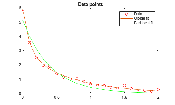
fprintf(['The residual norm at the good ending point is %f,' ...
   ' and the residual norm at the bad ending point is %f.'], ...
   fval,fvalbad)

The residual norm at the good ending point is 0.147723, and the residual norm at the bad ending point is 2.217300.