optimvalues
Description
val = optimvalues(prob,dataname1,dataval1,...)OptimizationValues
object for the problem prob. Specify all variable names and their
associated values, and optionally objective or constraint values, by using name-value
arguments. For example, to specify that x takes odd values from 1 through
99,
val = optimvalues(prob,x=1:2:99);
Use val as an initial point or initial population for
prob.
Examples
To create initial points for ga (genetic algorithm solver) in the problem-based approach, create an OptimizationValues object using optimvalues.
Create optimization variables for a 2-D problem with Rosenbrock's function as the fitness (objective) function.
x = optimvar("x",LowerBound=-5,UpperBound=5);
y = optimvar("y",LowerBound=-5,UpperBound=5);
rosenbrock = (10*(y - x.^2)).^2 + (1-x).^2;
prob = optimproblem(Objective=rosenbrock);
Create 100 random 2-D points within the bounds. The points must be row vectors.
rng default % For reproducibility
xval = -5 + 10*rand(1,100);
yval = -5 + 10*rand(1,100);
Create the initial point values object. Because you do not calculate the fitness values, the values appear as NaN in the display.
vals = optimvalues(prob,x=xval,y=yval)
vals =
  1×100 OptimizationValues vector with properties:

   Variables properties:
            x: [3.1472 4.0579 -3.7301 4.1338 1.3236 -4.0246 -2.2150 0.4688 4.5751 4.6489 -3.4239 4.7059 4.5717 -0.1462 3.0028 -3.5811 -0.7824 4.1574 2.9221 4.5949 1.5574 -4.6429 3.4913 4.3399 1.7874 2.5774 2.4313 -1.0777 1.5548 -3.2881 … ] (1×100 double)
            y: [-3.3782 2.9428 -1.8878 0.2853 -3.3435 1.0198 -2.3703 1.5408 1.8921 2.4815 -0.4946 -4.1618 -2.7102 4.1334 -3.4762 3.2582 0.3834 4.9613 -4.2182 -0.5732 -3.9335 4.6190 -4.9537 2.7491 3.1730 3.6869 -4.1556 -1.0022 -2.4013 … ] (1×100 double)

   Objective properties:
    Objective: [NaN NaN NaN NaN NaN NaN NaN NaN NaN NaN NaN NaN NaN NaN NaN NaN NaN NaN NaN NaN NaN NaN NaN NaN NaN NaN NaN NaN NaN NaN NaN NaN NaN NaN NaN NaN NaN NaN NaN NaN NaN NaN NaN NaN NaN NaN NaN NaN NaN NaN NaN NaN NaN NaN NaN … ] (1×100 double)
Solve the problem using ga starting from the initial point vals. Set ga options to have a population of 100.
opts = optimoptions("ga",PopulationSize=100);
[sol,fv] = solve(prob,vals,Solver="ga",Options=opts)
Solving problem using ga.
ga stopped because it exceeded options.MaxGenerations.
sol = struct with fields:
    x: 1.0551
    y: 1.1133
fv =
0.0030
ga returns a solution very near the true solution x = 1, y = 1 with a fitness value near 0.
To create initial points for surrogateopt in the problem-based approach, create an OptimizationValues object using optimvalues.
Create optimization variables for a 2-D problem with Rosenbrock's function as the objective function.
x = optimvar("x",LowerBound=-5,UpperBound=5);
y = optimvar("y",LowerBound=-5,UpperBound=5);
rosenbrock = (10*(y - x.^2)).^2 + (1 - x).^2;
prob = optimproblem(Objective=rosenbrock);
Create constraints that the solution is in a disc of radius 2 about the origin and lies below the line y = 1 + x.
disc = x^2 + y^2 <= 2^2;
prob.Constraints.disc = disc;
line = y <= 1 + x;
prob.Constraints.line = line;
Create 40 random 2-D points within the bounds. The points must be row vectors.
rng default % For reproducibility
N = 40;
xval = -5 + 10*rand(1,N);
yval = -5 + 10*rand(1,N);
Evaluate Rosenbrock's function on the random points. The function values must be a row vector. This step is optional. If you do not provide the function values, surrogateopt evaluates the objective function at the points (xval,yval). When you have the function values, you can save time for the solver by providing the values as data.
fval = zeros(1,N);
for i = 1:N
    p0 = struct('x',xval(i),'y',yval(i));
    fval(i) = evaluate(rosenbrock,p0);
end
Evaluate the constraints on the points. The constraint values must be row vectors. This step is optional. If you do not provide the constraint values, surrogateopt evaluates the constraint functions at the points (xval,yval).
discval = zeros(1,N);
lineval = zeros(1,N);
for i = 1:N
    p0 = struct('x',xval(i),'y',yval(i));
    discval(i) = infeasibility(disc,p0);
    lineval(i) = infeasibility(line,p0);
end
Create the initial point values object.
vals = optimvalues(prob,x=xval,y=yval,Objective=fval,disc=discval,line=lineval)
vals =
  1×40 OptimizationValues vector with properties:

   Variables properties:
            x: [3.1472 4.0579 -3.7301 4.1338 1.3236 -4.0246 -2.2150 0.4688 4.5751 4.6489 -3.4239 4.7059 4.5717 -0.1462 3.0028 -3.5811 -0.7824 4.1574 2.9221 4.5949 1.5574 -4.6429 3.4913 4.3399 1.7874 2.5774 2.4313 -1.0777 1.5548 -3.2881 … ] (1×40 double)
            y: [-0.6126 -1.1844 2.6552 2.9520 -3.1313 -0.1024 -0.5441 1.4631 2.0936 2.5469 -2.2397 1.7970 1.5510 -3.3739 -3.8100 -0.0164 4.5974 -1.5961 0.8527 -2.7619 2.5127 -2.4490 0.0596 1.9908 3.9090 4.5929 0.4722 -3.6138 -3.5071 … ] (1×40 double)

   Objective properties:
    Objective: [1.1067e+04 3.1166e+04 1.2698e+04 1.9992e+04 2.3846e+03 2.6593e+04 2.9811e+03 154.8722 3.5498e+04 3.6362e+04 1.9515e+04 4.1421e+04 3.7452e+04 1.1541e+03 1.6457e+04 1.6510e+04 1.5914e+03 3.5654e+04 5.9109e+03 5.7015e+04 … ] (1×40 double)

   Constraints properties:
         disc: [6.2803 13.8695 16.9638 21.8023 7.5568 12.2078 1.2024 0 21.3146 24.0987 12.7394 21.3751 19.3057 7.4045 19.5331 8.8248 17.7486 15.8313 5.2656 24.7413 4.7390 23.5542 8.1927 18.7982 14.4752 23.7379 2.1343 10.2207 10.7168 … ] (1×40 double)
         line: [0 0 5.3853 0 0 2.9222 0.6709 0 0 0 0.1841 0 0 0 0 2.5648 4.3798 0 0 0 0 1.1938 0 0 1.1217 1.0155 0 0 0 0 0.3467 1.2245 4.3736 0.9735 7.3213 0 0 0 0 3.3884]
Solve the problem using surrogateopt starting from the initial point vals.
[sol,fv] = solve(prob,vals,Solver="surrogateopt")Solving problem using surrogateopt.
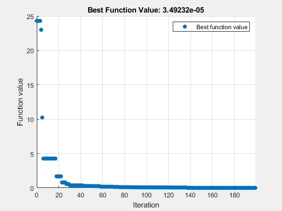
surrogateopt stopped because it exceeded the function evaluation limit set by
'options.MaxFunctionEvaluations'.
sol = struct with fields:
    x: 1.0031
    y: 1.0057
fv =
3.4923e-05
surrogateopt returns a solution somewhat near the true solution x = 1, y = 1 with an objective function value near 0.
Input Arguments
Name-Value Arguments
Output Arguments
Version History
Introduced in R2022aSee Also
Topics
- Specify Start Points for MultiStart, Problem-Based (Global Optimization Toolbox)
- Specify Starting Points and Values for surrogateopt, Problem-Based (Global Optimization Toolbox)
- Problem-Based Optimization Workflow