Estimate Target Position using MIMO Radar
A distributed MIMO radar system with two transmit anchors and five receive anchors measures the TSOA from each transmit-receive anchor pairs. Then, the radar system applies the two-step WLLS algorithm using the TSOA estimates and anchor positions. The data is loaded from TSOAEstimatorExampleData, whose variables are listed here:
Parameter | Description | Size |
|---|---|---|
tsoaest | TSOA estimates | 2-by-5 |
tsoavar | TSOA estimate variance | 2-by-5 |
txpos | Transmit anchor positions | 3-by-2 |
rxpos | Receive anchor positions | 3-by-5 |
tgtpos | True target position | 3-by-1 |
First, load data from mat-file.
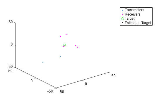
load TSOAEstimatorExampleDataDraw the positions of the transmitters and receivers.
plot3(txpos(1,:),txpos(2,:),txpos(3,:),'.')
a = 50;
axis([-a a -a a -a a])
hold on
plot3(rxpos(1,:),rxpos(2,:),rxpos(3,:),'m.')
plot3(tgtpos(1,:),tgtpos(2,:),tgtpos(3,:),'go')
Estimate and plot the target position.
[tgtposest,tgtposcov] = tsoaposest(tsoaest,tsoavar,txpos,rxpos);
plot3(tgtposest(1,:),tgtposest(2,:),tgtposest(3,:),'.k')
legend('Transmitters','Receivers','Target','Estimated Target')
RMSE of target position estimate.
rmsepos = rmse(tgtposest,tgtpos);
disp(['RMS TSOA positioning error = ',num2str(rmsepos),' meters.'])
RMS TSOA positioning error = 0.1131 meters.
See Also
Radar
Designer (Radar Toolbox) | phased.Receiver | phased.Transmitter | radarbudgetplot (Radar Toolbox)