Main Content

lyapunovExponent

Characterize the rate of separation of infinitesimally close trajectories

Description

example

lyapExp = lyapunovExponent(X,fs) estimates the Lyapunov exponent of the uniformly sampled time-domain signal X using sampling frequency fs. Use lyapunovExponent to characterize the rate of separation of infinitesimally close trajectories in phase space to distinguish different attractors. Lyapunov exponent is useful in quantifying the level of chaos in a system, which in turn can be used to detect potential faults.

example

lyapExp = lyapunovExponent(X,fs,lag) estimates the Lyapunov exponent for the time delay lag.

example

lyapExp = lyapunovExponent(X,fs,[],dim) estimates the Lyapunov exponent for the embedding dimension dim.

example

lyapExp = lyapunovExponent(X,fs,lag,dim) estimates the Lyapunov exponent for the time delay lag and embedding dimension dim.

example

[lyapExp,estep,ldiv] = lyapunovExponent(___) estimates the Lyapunov exponent, expansion step, and the corresponding logarithmic divergence of the uniformly sampled time-domain signal X. Use expansion step estep and the corresponding logarithmic divergence ldiv for signal diagnostics.

example

___ = lyapunovExponent(___,Name,Value) estimates the Lyapunov exponent with additional options specified by one or more Name,Value pair arguments.

example

lyapunovExponent(___) with no output arguments creates an average logarithmic divergence versus expansion step plot.

Use the generated interactive plot to find an appropriate ExpansionRange.

Examples

collapse all

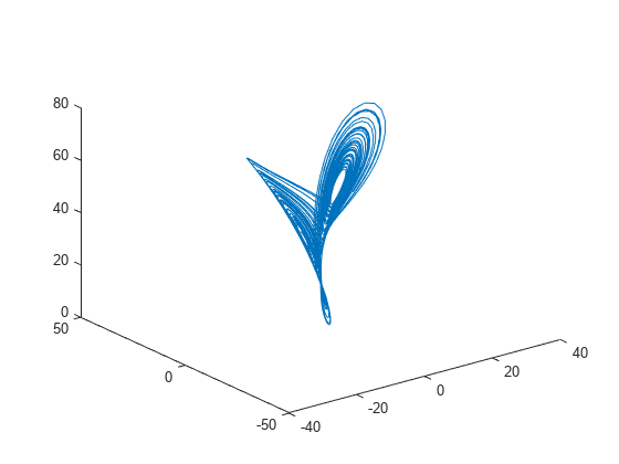
In this example, consider a Lorenz attractor describing a unique set of chaotic solutions.

Load the data set and sampling frequency fs to the workspace, and visualize the Lorenz attractor in 3-D.

load('lorenzAttractorExampleData.mat','data','fs');
plot3(data(:,1),data(:,2),data(:,3));

For this example, use the x-direction data of the Lorenz attractor. Since Lag is unknown, estimate the delay using phaseSpaceReconstruction. Set dimension to 3 since the Lorenz attractor is a three-dimensional system. The dim and lag parameters are required to create the logarithmic divergence versus expansion step plot.

xdata = data(:,1);
dim = 3;
[~,lag] = phaseSpaceReconstruction(xdata,[],dim)
lag = 10

Create the average logarithmic divergence versus expansion step plot for the Lorenz attractor, using the lag value obtained in the previous step. Set a sufficiently large expansion range to capture all the expansion steps.

eRange = 200;
lyapunovExponent(xdata,fs,lag,dim,'ExpansionRange',eRange)

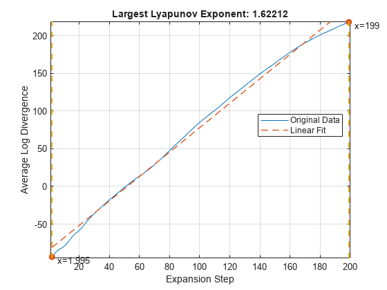
The first dashed, vertical green line (on the left) indicates the minimum number of steps used to estimate the expansion range, while the second vertical green line (on the right), represents the maximum number of steps used. Together, the first and second vertical lines represent the expansion range. The dashed red line indicates the linear fit line for the data, within the expansion range.

To compute the largest Lyapunov exponent, you first need to determine the expansion range needed for accurate estimation.

In the plot, drag the two dashed, vertical green lines to best fit the linear fit line to the original data line to obtain the expansion range: Kmin and Kmax.

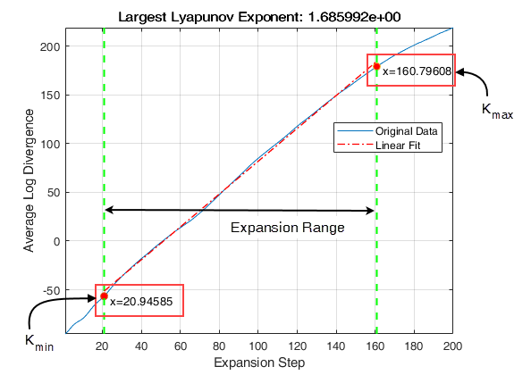
Note the new values of the expansion range after dragging the two vertical lines for an appropriate fit.

Since expansion range can only be specified using whole numbers, round-off Kmin and Kmax to the nearest integer. Find the largest Lyapunov exponent of the Lorenz attractor using the new expansion range value.

Kmin = 21;
Kmax = 161;
lyapExp = lyapunovExponent(xdata,fs,lag,dim,'ExpansionRange',[Kmin Kmax])
lyapExp = 1.6834

A negative Lyapunov exponent indicates convergence, while positive Lyapunov exponents demonstrate divergence and chaos. The magnitude of lyapExp is an indicator of the rate of convergence or divergence of the infinitesimally close trajectories.

Input Arguments

collapse all

Uniformly sampled time-domain signal, specified as a vector, array, or timetable. If X has multiple columns, lyapunovExponent computes the largest Lyapunov exponent by treating X as a multivariate signal.

If X is specified as a row vector, lyapunovExponent treats it as a univariate signal.

Sampling frequency, specified as a scalar. Sampling frequency or sampling rate is the average number of samples obtained in one second.

If fs is not supplied, a normalized frequency of 2π is used to compute the Lyapunov exponent. If X is specified as a timetable, the sampling time is inferred from it.

Embedding dimension, specified as a scalar or vector. dim is equivalent to the 'Dimension' name-value pair.

Time delay, specified as a scalar or vector. lag is equivalent to the 'Lag' name-value pair.

Name-Value Arguments

Specify optional pairs of arguments as Name1=Value1,...,NameN=ValueN, where Name is the argument name and Value is the corresponding value. Name-value arguments must appear after other arguments, but the order of the pairs does not matter.

Before R2021a, use commas to separate each name and value, and enclose Name in quotes.

Example: …,'Dimension',3

Embedding dimension, specified as the comma-separated pair consisting of 'Dimension' and either a scalar or vector. When Dimension is scalar, every column in X is reconstructed using Dimension. When Dimension is a vector having same length as the number of columns in X, the reconstruction dimension for column i is Dimension(i).

Specify Dimension based on the dimension of your system, that is, the number of states. For more information on embedding dimension, see phaseSpaceReconstruction.

Delay in phase space reconstruction, specified as the comma-separated pair consisting of 'Lag' and either a scalar or vector. When Lag is scalar, every column in X is reconstructed using Lag. When Lag is a vector having same length as the number of columns in X, the reconstruction delay for column i is Lag(i).

The default value of Lag is 1.

If the delay is too small, random noise is introduced in the data. In contrast, if the lag is too large, the reconstructed dynamics do not represent the true dynamics of the time series. For more information on estimating optimal delay, see phaseSpaceReconstruction.

Mean period, specified as the comma-separated pair consisting of 'MinSeparation' and a positive scalar integer.

MinSeparation is the threshold value used to find the nearest neighbor i* for a point i to estimate the largest Lyapunov exponent.

The default value of MinSeparation is ceil(fs/max(meanfreq(X,fs))).

Range of expansion steps, specified as the comma-separated pair consisting of 'ExpansionRange' and either a 1x2 positive integer array or a positive scalar integer.

The minimum and maximum value of ExpansionRate is used to estimate the local expansion rate to calculate the Lyapunov exponent.

If ExpansionRange is specified as a scalar M, then the range is set to be [1, M]. ExpansionRange can only be specified using positive whole numbers and the default value is [1, 5].

Output Arguments

collapse all

Largest Lyapunov exponent, returned as a scalar. lyapExp quantifies the rate of divergence or convergence of close trajectories in phase space.

A negative Lyapunov exponent indicates convergence, while positive Lyapunov exponents demonstrate divergence and chaos. The magnitude of lyapExp is an indicator of the rate of convergence or divergence of the infinitesimally close trajectories.

The ability to discern levels of divergence within data sets is useful in the field of engineering to estimate component failure by studying their vibration and acoustic signals, or to predict when a ship would capsize based on its motion.[2][3]

Expansion step used for estimation, returned as an array. estep is the difference between the maximum and minimum expansion range split into an equal number of points defined by the maximum value of ExpansionRange.

Logarithmic divergence, returned as an array with the same size as estep. The magnitude of each value in ldiv corresponds to the logarithmic convergence or divergence of each point in estep.

Algorithms

Lyapunov exponent is calculated in the following way:

  1. The lyapunovExponent function first generates a delayed reconstruction Y1:N with embedding dimension m, and lag τ.

  2. For a point i, the software then finds the nearest neighbor point i* that satisfies mini*YiYi* such that |ii*|>MinSeparation, where MinSeparation, the mean period, is the reciprocal of the mean frequency.

  3. From [1], the Lyapunov exponent for the entire expansion range is calculated as,

    λ(i)=1(KmaxKmin+1)dtK=KminKmax1KlnYi+KYi*+KYiYi*

    where, Kmin and Kmax represent ExpansionRange, dt is the sampling time and ldiv=lnYi+KYi*+KYiYi*

  4. A single value for the Lyapunov exponent is then calculated from the earlier step using the polyfit command as,

    lyapExp = polyfit([Kmin Kmax],λ(i))

References

[1] Michael T. Rosenstein , James J. Collins , Carlo J. De Luca. "A practical method for calculating largest Lyapunov exponents from small data sets ". Physica D 1993. Volume 65. Pages 117-134.

[2] Caesarendra, Wahyu & Kosasih, P & Tieu, Kiet & Moodie, Craig. "An application of nonlinear feature extraction-A case study for low speed slewing bearing condition monitoring and prognosis." IEEE/ASME International Conference on Advanced Intelligent Mechatronics: Mechatronics for Human Wellbeing, AIM 2013.1713-1718. 10.1109/AIM.2013.6584344.

[3] McCue, Leigh & W. Troesch, Armin. (2011). "Use of Lyapunov Exponents to Predict Chaotic Vessel Motions". Fluid Mechanics and its Applications. 97. 415-432. 10.1007/978-94-007-1482-3_23.

Extended Capabilities

Version History

Introduced in R2018a