Radar Design Part II: From Radar Data to IQ Signal Synthesis

Since R2024b

This example shows how to easily go from a measurement-level model of a radar to a waveform-level radar transceiver that can model IQ samples. Radar Design Part I: From Power Budget Analysis to Dynamic Scenario Simulation demonstrates how you can configure a radar in the Radar Designer app as in Radar Link Budget Analysis and then export a script that creates a measurement-level, statistics-based model and dynamic radar scenario. Part II shows how to go from the measurement-level model to the waveform-level model as well as tips to help you better use this pipeline and how to process the raw radar data. Lastly, this example compares the performance of all three model fidelities (power-level, measurement-level, waveform-level) by using the results from Part I of this series. This pipeline allows you to efficiently test your radar hardware and software designs at multiple levels of fidelity and see their performance on tasks like detection and tracking.

Data Synthesis with a Measurement-Level Radar Model

In Radar Design Part I: From Power Budget Analysis to Dynamic Scenario Simulation, you learned how to export a MATLAB script that creates a radarDataGenerator and a radarScenario. This example starts by loading a script that was previously exported using the Export Radar Data Generator MATLAB Script option from the Export tab in the Radar Designer app. Run the following lines to simulate the measurement-level radar to fill your workspace with the necessary variables.

rng('default')
run("Part_I_EXPORT_Swerling1.m")

Create a Waveform-Level Radar Transceiver to Generate IQ Samples

You can extend the design process to waveform-level simulation by creating a radarTransceiver object from the radarDataGenerator. To see this, we first define four stationary targets with the function, helperCreateTargets. This function was also used in Part I of this example series. Then, configure a staring radar with a wide field of view. Disable the elevation resolution to simplify the radar transceiver and speed up the simulation time. Recognize that because all the targets are static, we only have to look in the static Doppler bin for the targets which greatly simplifies detection later on.

In this section, the radarTransceiver derives its parameters directly from the radarDataGenerator in order to create a radar model with equivalent performance. However, because the radarDataGenerator abstracts away much of the information from the Radar Designer app, some of the radar properties of this radarTransceiver do not match those described in the app. Despite this, the newly created radar transceiver is still equivalent to the radarDataGenerator (up to noise). This is possible because many different radar configurations can result in the same processing gain.

release(radarSensorModel)                                        % Allows modification of the radar
radarSensorModel.HasElevation = false;                           % Simplifies the scenario and allows for faster processing
radarSensorModel.AzimuthResolution = radarSensorModel.FieldOfView(1); % Obviates beamforming
radarSensorModel.HasRangeAmbiguities  = true;
% Ambiguities are set again for higher precision than exported radar struct
radarSensorModel.MaxUnambiguousRange = time2range(1/radar.PRF);
radarSensorModel.MaxUnambiguousRadialSpeed = freq2wavelen(radar.Frequency)*radar.PRF/4; 

sensorIQ = radarTransceiver(radarSensorModel)                    % Create radar transceiver

sensorIQ = 
  radarTransceiver with properties:

                Waveform: [1x1 phased.RectangularWaveform]
             Transmitter: [1x1 phased.Transmitter]
         TransmitAntenna: [1x1 phased.Radiator]
          ReceiveAntenna: [1x1 phased.Collector]
                Receiver: [1x1 phased.ReceiverPreamp]
      MechanicalScanMode: 'None'
      ElectronicScanMode: 'None'
        MountingLocation: [0 0 0]
          MountingAngles: [0 -3 0]
    NumRepetitionsSource: 'Property'
          NumRepetitions: 20
       RangeLimitsSource: 'Property'
             RangeLimits: [0 400000]
         RangeOutputPort: false
          TimeOutputPort: false

Important Notes on Rounding Error and Matched Filter Length

• The exported MATLAB script rounds some radar properties to a precision of six significant figures for readability which may cause subtle changes in the waveform-level model created from the measurement-level model. For non-integer intrinsic radar properties, it is best practice to recompute those values and avoid any rounding.

• Make sure that Receiver.SampleRate * Waveform.PulseWidth equals an integer number of samples. If that is not the case, the waveform-level results may not match the measurement-level results.

% Create a scenario for the radarTransceiver
scene = radarScenario('UpdateRate',0); % UpdateRate of 0 updates when new measurements are available

% Place radar on a stationary platform
radarPos = [0,0,radar.Height]; % East-North-Up Cartesian Coordinates
radarOrientation = [0 0 0];  % (deg) Yaw, Pitch, Roll
radarPlat = platform(scene,'Position',radarPos,'Sensors',sensorIQ,'Orientation',radarOrientation);

% Define Static Targets
[tgt1, tgt2, tgt3, tgt4] = helperCreateTargets(scene);
tgts = [tgt1 tgt2 tgt3 tgt4];

Straddle or scalloping loss accounts for the loss when a target is not in the center of a range or Doppler bin. This loss is not modeled by the radarDataGenerator. As a result, the radarDataGenerator always assumes the best-case scenario, i.e. that the targets are in the middle of the range-Doppler Bins. The impact of this nonideality is usually no more than 3 dB each in the range and Doppler dimensions. Thus, in order to facilitate a more precise comparison between the three levels of fidelity, we move the targets slightly so that they are in the middle of their range bins using the function helperMoveTarget2BinCenters. The resulting change in range is very small and has a minimal impact on the SNR.

% Place targets at the center of range the radar's range bins to remove
% straddle loss
helperMoveTarget2BinCenters(tgts,radarSensorModel,sensorIQ,radarPlat)

Matched Filter and Computing the Range-Doppler Response

To maximize the SNR and process the raw data, use a matched filter in the phased.RangeDopplerResponse System object™.

% Create Matched Filter
coeff = getMatchedFilter(sensorIQ.Waveform);
fs = sensorIQ.Waveform.SampleRate;
fc = sensorIQ.TransmitAntenna.OperatingFrequency;

% Get the range-Doppler response
rgdpResp = phased.RangeDopplerResponse(SampleRate=fs,DopplerOutput="Speed",OperatingFrequency=fc);
[sig, ~] = receive(scene);
sig = sig{1};

[Xrgdp,rgGrid,~] = rgdpResp(sig,coeff);
powerSpectrum = pow2db(abs(Xrgdp).^2);

Noise Power and Plotting the Static Range-Doppler Response

Because both the radar and targets are static, searching for targets in the static Doppler bin is sufficient for detecting the present targets. The first step in this detection process is to calculate the noise power in the processed signal which is eventually used as an input to the detection threshold. This noise power can be computed using knowledge about the radar properties and various processing gains associated with the signal processing.

npower = noisepow(sensorIQ.Receiver.SampleRate,sensorIQ.Receiver.NoiseFigure,sensorIQ.Receiver.ReferenceTemperature);
PndB = pow2db(npower);                  % Noise Power at output of receiver
Gmf = pow2db(coeff'*coeff);             % Gain from matched filter
Gdp = pow2db(sensorIQ.NumRepetitions);  % Gain from Doppler processing
PndB = PndB + Gmf + Gdp                 % Total noise power in dB           

PndB = 
-129.2040

An alternative way that you can compute the noise floor without having to know each processing step or radar property is by creating an empty signal (all zeros) and feeding it through the same processing pipeline as the simulated signal and then computing the average power of the output.

rcvr = clone(sensorIQ.Receiver);
Xnoise = rcvr(zeros(size(sig)));
Xnoise = rgdpResp(Xnoise,coeff);
PndB_Estimated = pow2db(mean(abs(Xnoise(:)).^2)) % Matches the value of PndB right above

PndB_Estimated = 
-129.2073

After the noise power is computed, an offset based on the probability of false alarms is added to the noise power to set the detection threshold.

threshold = PndB + npwgnthresh(radar.Pfa) % Threshold for detecting targets

threshold = 
-117.8003

% Plot the Static Doppler Bin 
staticIdx = floor(size(powerSpectrum,2)/2)+1; % Middle bin in slow time
c = physconst('lightspeed');
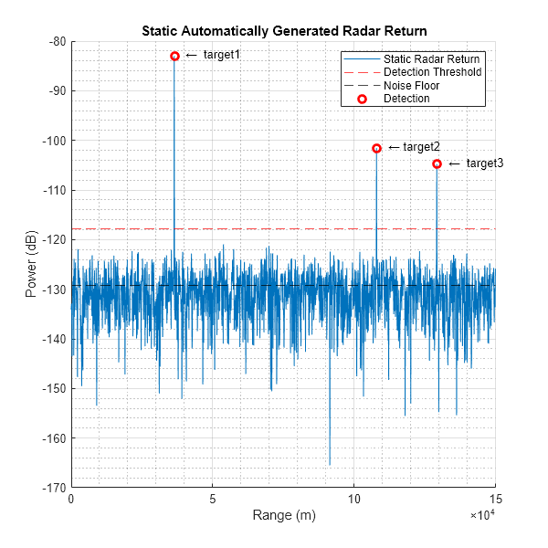
detectedPower = plotDopplerBin(sensorIQ, powerSpectrum, rgGrid, staticIdx, PndB, threshold, c);
title("Static Automatically Generated Radar Return")

Notice that just like in Part I of this series, target 4 was not detected because its reflection was below the noise floor.

% Save for comparison later
IQStaringSNR = detectedPower - PndB;
IQStaringTargetIdx = [1;2;3];

Align Power-Level and Waveform-Level Models

As mentioned in the preceding section, because the radarDataGenerator abstracts away many of the properties of the Radar Designer app, the automatically created radarTransceiver object does not necessarily match all of the properties of the radar designed in the app. This is possible because there are many different radar configurations that can result in the same processing gains and resolutions. Despite this, we show how one can easily adjust the automatically generated radar transceiver so that it is aligned with the Radar Designer app. While different configurations may require you to change other properties of the radar transceiver, this serves as an example on how to get started.

appEquivIQ = radarTransceiver(radarSensorModel);    % Default construction of the radar transceiver
appEquivIQ.Transmitter.PeakPower = radar.PeakPower; % Match peak power
appEquivIQ.Receiver.LossFactor = radar.CustomLoss;  % Apply custom loss to receiver
appEquivIQ.Receiver.NoiseFigure = pow2db(radar.NoiseTemperature/radar.ReferenceNoiseTemperature); % Match noise figure

% Tx and Rx antennas share the same handle so we only have change it once
% The same gain is used for both Tx and RX
appEquivIQ.TransmitAntenna.Sensor.MagnitudePattern = appEquivIQ.TransmitAntenna.Sensor.MagnitudePattern + radar.Gain(1);

Waveform

Although the Radar Designer app does not specify the waveform, certain configurations may necessitate changing the waveform from the default rectangular pulse. Because the radar transceiver assumes a rectangular waveform, the generated waveform has a pulse width of 0.67 microseconds and a bandwidth of 1.5 MHz. Both of these correspond to the correct range resolution of 99.93 meters.

bw2rangeres(sensorIQ.Waveform.bandwidth, c)

time2range(sensorIQ.Waveform.PulseWidth)

However, the pulsewidth specified in the app is 2 microseconds which would not allow the range resolution to be so precise with a rectangular pulse. To rectify this, we can change the waveform to a linear frequency modulated (LFM) chirp as seen below in order to accommodate both the range resolution and the pulse width. LFM waveforms' range resolution does not depend on pulse width but instead just the sweep bandwidth. This advantage among others can be visualized using the ambiguity function explained in Waveform Analysis Using the Ambiguity Function.

wfm = phased.LinearFMWaveform("SweepBandwidth",radar.PulseBandwidth,'PulseWidth',radar.Pulsewidth,'SampleRate',appEquivIQ.Receiver.SampleRate,'PRF',radar.PRF,SweepInterval='Symmetric');
appEquivIQ.Waveform = wfm;

Simulation

Create a radar scenario and place a stationary radar platform and stationary targets in it.

scene = radarScenario('UpdateRate',0); % UpdateRate of 0 updates when new measurements are available

% Place radar on a stationary platform
radarPos = [0,0,radar.Height]; % East-North-Up Cartesian Coordinates
radarOrientation = [0 0 0];  % (deg) Yaw, Pitch, Roll
radarPlat = platform(scene,'Position',radarPos,'Sensors',appEquivIQ,'Orientation',radarOrientation);

% Define Static Targets
[tgt1, tgt2, tgt3, tgt4] = helperCreateTargets(scene);
tgts = [tgt1 tgt2 tgt3 tgt4];

% Place targets at the center of range the radar's range bins to remove
% straddle loss
helperMoveTarget2BinCenters(tgts,radarSensorModel,appEquivIQ, radarPlat)

Calculate noise power and plot the static range-Doppler response.

% Create Matched Filter
coeff = getMatchedFilter(appEquivIQ.Waveform);
fs = appEquivIQ.Waveform.SampleRate;
fc = appEquivIQ.TransmitAntenna.OperatingFrequency;

% Get the range-Doppler response
rgdpResp = phased.RangeDopplerResponse(SampleRate=fs,DopplerOutput="Speed",OperatingFrequency=fc);
[sig, ~] = receive(scene);
sig = sig{1};

[Xrgdp,rgGrid,dpGrid] = rgdpResp(sig,coeff);
powerSpectrum = pow2db(abs(Xrgdp).^2);

Noise Power and Plotting the Static Range-Doppler Response

rcvr = clone(appEquivIQ.Receiver);
Xnoise = rcvr(zeros(size(sig)));
Xnoise = rgdpResp(Xnoise,coeff);
PndB_Estimated_App = pow2db(mean(abs(Xnoise(:)).^2));
threshold = PndB_Estimated_App + npwgnthresh(radar.Pfa);

% Plot the Static Doppler Bin 
staticIdx = floor(size(powerSpectrum,2)/2)+1;
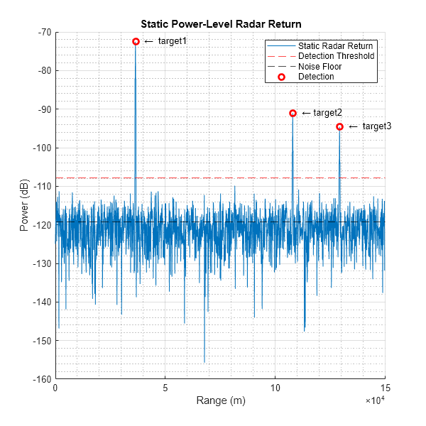
detectedPowerApp = plotDopplerBin(appEquivIQ, powerSpectrum, rgGrid, staticIdx, PndB_Estimated_App, threshold, c);
title("Static Power-Level Radar Return")

Similar to the results in Part I, the fourth target is blow the detection threshold.

% Save for comparison later
IQStaringAppSNR = detectedPowerApp - PndB_Estimated_App;
IQStaringAppTargetIdx = [1;2;3];

Abbreviated List of the Inherited Properties of the Radar Transceiver

As we just showed above, there are multiple radar configurations that result in equivalent measurement-level radar models. While the behavior of the radar transceivers may be the same in many aspects, in some cases it may be important to align the radar transceiver to the app. Below is an abbreviated list of the properties from the app that are either automatically inferred from the measurement-level model or that need to be adjusted to match the value set in the app.

Property	Location in radarTransceiver Object	Automatic generation of the radarTransceiver (sensorIQ)	Adjusted generation of the radarTransceiver (appEquivIQ)
Number of Pulses	radarTransceiver.NumRepetitions	Matches value in app	Matches value in app
Waveform Type	radarTransceiver.Waveform	Defaults to phased.RectangularWaveform	phased.LinearFMWaveform
Bandwidth	radarTransceiver.Waveform.SweepBandwidth	Matches value in app	Matches value in app
Sample Rate	radarTransceiver.Waveform.SampleRate	Matches bandwidth in app	Matches bandwidth in app
PRF	radarTransceiver.Waveform.PRF	Matches value in app	Matches value in app
Pulse Width	radarTransceiver.Waveform.PulseWidth	Assumes limit from rectangular waveform	Matches value in app
Antenna Gain	radarTransceiver.TransmitAntenna.Sensor.MagnitudePattern radarTransceiver.ReceiveAntenna.Sensor.MagnitudePattern	Set to 0 dB by default. Gain is absorbed in peak power.	Matches value in app
Custom Loss	radarTransceiver.Receiver.LossFactor	Set to 0 by default. Loss is absorbed in peak power.	Matches the custom loss from the app
Peak Power	radarTransceiver.Transmitter.PeakPower	Combines many gains and losses into power	Matches value in app
Frequency	radarTransceiver.TransmitAntenna.OperatingFrequency radarTransceiver.ReceiveAntenna.OperatingFrequency	Matches value in app	Matches value in app

Compare the Results of the Three Levels of Fidelity

Here we compare the SNRs of the app and the 4 radar models:

1. Radar Designer App

2. Measurement-Level Staring Radar

3. Measurement-Level Scanning Radar

4. Waveform-level Radar (default construction with rectangular pulse)

5. Waveform-level Radar (aligned to power-level design)

The first three items in this list were already computed in Part I of this series and are displayed and saved at the end of that example.

% Get the SNR and Target Index of the statistical Model results
AppAndStatResults = load('AppAndStatResults.mat').results;
AppAndStatLabels = load('AppAndStatResults.mat').labels;

% Create the Figure
figure
bar(["Target 1","Target 2","Target 3","Target 4\newline(Undetected)",],[AppAndStatResults [IQStaringSNR(IQStaringTargetIdx);NaN] [IQStaringAppSNR(IQStaringAppTargetIdx);NaN]])
yline(npwgnthresh(radar.Pfa),'LineWidth',2,'LineStyle','--')
ylabel('SNR (dB)')
title('Comparing Target SNR For Each Simulation Type')
grid
grid minor
legend([AppAndStatLabels,"Waveform-Level Default","Waveform-Level Power-Aligned","SNR Detection Threshold"])

Summary

In this example we saw how to go from a measurement-level radar to a waveform-level radar. Notably, we got a closer look at how defaults in this conversion process might create a radar that differs from the radar originally designed in the Radar Designer app. This makes sense because the measurement-level radar model abstracts away much of the information related to the waveform and hardware of the radar. Despite this, the automatically created radar transceiver still performs identically to the measurement-level and power-level models up to noise. Then we showed how we can change just a few properties in the radar transceiver so that it matches the radar designed in the app. Lastly, we showed that both radar transceivers perform very closely to the power-level and measurement-level radar models described in Part I of this example series.

Helper Functions

% Define targets in the scenario (same as in Part I of this example series)
function [tgt1, tgt2, tgt3, tgt4] = helperCreateTargets(scene)
    tgt1 = platform(scene, ...
        'ClassID',1, ... % set to 1 for targets
        'Position',[30e3 20e3 5e3], ...
        'Signatures',{rcsSignature(Pattern=5)}); % (dBsm)
    tgt2 = platform(scene, ...
        'ClassID',1, ...
        'Position',[95e3 -50e3 10e3], ...
        'Signatures',{rcsSignature(Pattern=5)}); % (dBsm)
    tgt3 = platform(scene, ...
        'ClassID',1, ...
        'Position',[125e3 30e3 12e3], ...
        'Signatures',{rcsSignature(Pattern=5)}); % (dBsm)
    tgt4 = platform(scene, ...
        'ClassID',1, ...
        'Position',[250e3 250e3 5e3], ...
        'Signatures',{rcsSignature(Pattern=5)}); % (dBsm)
end

% Compensates for straddle loss by shifting targets to the centers of the
% relevant range bins
function helperMoveTarget2BinCenters(tgts,radarSensorModel,radarTransceiverModel, radarPlatform)
    pos = targetPoses(radarPlatform); % Target locations relative to radar sensor platform
    pos = reshape([pos.Position],3,[]) - radarSensorModel.MountingLocation'; % Target locations relative to radar radar antenna
    [th,ph,rgs] = cart2sph(pos(1,:),pos(2,:),pos(3,:));
    rbins = round(range2time(rgs)*radarTransceiverModel.Waveform.SampleRate); % Round to nearest range bin
    rgs = time2range(rbins/radarTransceiverModel.Waveform.SampleRate); 
    [x,y,z] = sph2cart(th,ph,rgs);
    for m = 1:numel(tgts)
        tgts(m).Trajectory.Position = [x(m) y(m) z(m)] + radarSensorModel.MountingLocation + radarPlatform.Position; % Place target at nearest integer multiple of a range bin
    end
end

% Plots the static Doppler bin (where targets are not moving)
function detectedPower = plotDopplerBin(sensorIQ, powerSpectrum, rgGrid, staticIdx, PndB, threshold, c)
    f = figure;
    f.Position(3:4) = [600 600];
    hold on
    plot(rgGrid,powerSpectrum(:,staticIdx),'DisplayName','Static Radar Return')
    yline(threshold,'r--','DisplayName','Detection Threshold')
    yline(PndB,'k--','DisplayName','Noise Floor')
    
    rangeRes = bw2rangeres(sensorIQ.Waveform.bandwidth , c);
    [detectedPower,detectedPeakBins] = findpeaks(powerSpectrum(:,staticIdx),'MinPeakHeight',threshold,'MinPeakDistance',10);
    detectedPeaks = rangeRes*detectedPeakBins;
    scatter(detectedPeaks,detectedPower,'ro','LineWidth',2,'DisplayName', 'Detection')
    text(detectedPeaks,detectedPower,{' \leftarrow target1',' \leftarrowtarget2',' \leftarrow target3'})
    legend
    xlabel('Range (m)')
    ylabel('Power (dB)')
    grid
    grid minor
end