Train PG Agent with Baseline to Control Discrete Action Space System
This example shows how to train a policy gradient (PG) agent with baseline to control a discrete action space second-order dynamic system modeled in MATLAB®.
For more information on the basic PG agent with no baseline, see the example Train PG Agent to Balance Cart-Pole System.
Discrete Action Space Double Integrator MATLAB Environment
The reinforcement learning environment for this example is a second-order double integrator system with a gain and a discrete action space. The training goal is to control the position of a mass in the second-order system by applying a force input.
For this environment:
The mass starts at an initial position between –2 and 2 units.
The force action signal from the agent to the environment is from –2 to 2 N.
The observations from the environment are the position and velocity of the mass.
The episode terminates if the mass moves more than 5 m from the original position or if .
The reward , provided at every time step, is a discretization of :
Here:
is the state vector of the mass.
is the force applied to the mass.
is the weights on the control performance; .
is the weight on the control effort; .
For more information on this model, see Load Predefined Control System Environments.
Create Double Integrator MATLAB Environment Interface
Create a predefined environment interface for the pendulum.
env = rlPredefinedEnv("DoubleIntegrator-Discrete")env =
DoubleIntegratorDiscreteAction with properties:
Gain: 1
Ts: 0.1000
MaxDistance: 5
GoalThreshold: 0.0100
Q: [2x2 double]
R: 0.0100
MaxForce: 2
State: [2x1 double]
The interface has a discrete action space where the agent can apply one of three possible force values to the mass: -2, 0, or 2 N.
Obtain the observation and action information from the environment interface.
obsInfo = getObservationInfo(env);
actInfo = getActionInfo(env);
Fix the random generator seed for reproducibility.
rng(0)
Create PG Agent Actor
For policy gradient agents, the actor executes a stochastic policy, which for discrete action spaces is approximated by a discrete categorical actor. This actor must take the observation signal as input and return a probability for each action.
To approximate the policy within the actor, use a neural network. Define the network as an array of layer objects with one input (the observation) and one output (the action), and get the dimension of the observation space and the number of possible actions from the environment specification objects. For more information on creating a deep neural network value function representation, see Create Policies and Value Functions.
actorNet = [
    featureInputLayer(obsInfo.Dimension(1))
    fullyConnectedLayer(numel(actInfo.Elements))
    ];
Convert to dlnetwork and display the number of weights.
actorNet = dlnetwork(actorNet);
summary(actorNet)
   Initialized: true

   Number of learnables: 9

   Inputs:
      1   'input'   2 features
Specify training options for the actor. For more information, see rlOptimizerOptions. Alternatively, you can change agent (including actor and critic) options using dot notation after the agent is created.
actorOpts = rlOptimizerOptions( ...
    LearnRate=5e-3, ...
    GradientThreshold=1);
Create the actor representation using the neural network and the environment specification objects. For more information, see rlDiscreteCategoricalActor.
actor = rlDiscreteCategoricalActor(actorNet,obsInfo,actInfo);
To return the probability distribution of the possible actions as a function of a random observation, and given the current network weights, use evaluate.
prb = evaluate(actor,{rand(obsInfo.Dimension)})prb = 1x1 cell array
{3x1 single}
prb{1}ans = 3x1 single column vector
0.4994
0.3770
0.1235
Create PG Agent Baseline
The PG Agent algorithm, (also known as REINFORCE) returns can be compared to a baseline that depends on the state. This can reduce the variance of the expected value of the update and thus improve the speed of learning. A possible choice for the baseline is an estimate of the state value function [1].
A value-function approximator object must accept an observation as input and return a single scalar (the estimated discounted cumulative long-term reward) as output. Use a neural network as approximation model. Define the network as an array of layer objects, and get the dimension of the observation space and the number of possible actions from the environment specification objects.
baselineNet = [
    featureInputLayer(obsInfo.Dimension(1))
    fullyConnectedLayer(8)
    reluLayer
    fullyConnectedLayer(1)
    ];
Convert to dlnetwork and display the number of weights.
baselineNet = dlnetwork(baselineNet);
Create the baseline value function approximator using baselineNet, and the observation specification. For more information, see rlValueFunction.
baseline = rlValueFunction(baselineNet,obsInfo);
Check the baseline with a random observation input.
getValue(baseline,{rand(obsInfo.Dimension)})ans = single
0.2152
Specify some training option for the baseline.
baselineOpts = rlOptimizerOptions( ...
    LearnRate=5e-3, ...
    GradientThreshold=1);
To create the PG agent with baseline, specify the PG agent options using rlPGAgentOptions and set the UseBaseline option set to true.
agentOpts = rlPGAgentOptions(...
    UseBaseline=true, ...
    ActorOptimizerOptions=actorOpts, ...
    CriticOptimizerOptions=baselineOpts);
Then create the agent using the specified actor representation, baseline representation, and agent options. For more information, see rlPGAgent.
agent = rlPGAgent(actor,baseline,agentOpts);
Check the agent with a random observation input.
getAction(agent,{rand(obsInfo.Dimension)})ans = 1x1 cell array
{[0]}
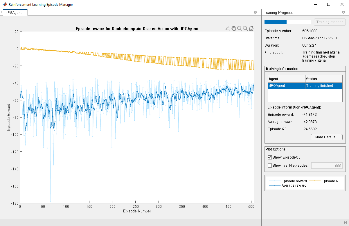
Train Agent
To train the agent, first specify the training options. For this example, use the following options.
Run at most 1000 episodes, with each episode lasting at most 200 time steps.
Display the training progress in the Reinforcement Learning Training Monitor dialog box (set the
Plotsoption) and disable the command line display (set theVerboseoption).Stop training when the agent receives a moving average cumulative reward greater than –43. At this point, the agent can control the position of the mass using minimal control effort.
For more information, see rlTrainingOptions.
trainOpts = rlTrainingOptions(...
    MaxEpisodes=1000, ...
    MaxStepsPerEpisode=200, ...
    Verbose=false, ...
    Plots="training-progress",...
    StopTrainingCriteria="AverageReward",...
    StopTrainingValue=-43);
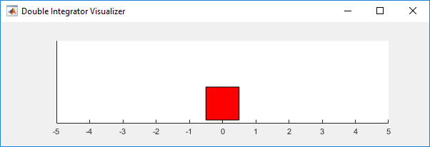
You can visualize the double integrator system using the plot function during training or simulation.
plot(env)

Train the agent using the train function. Training this agent is a computationally intensive process that takes several minutes to complete. To save time while running this example, load a pretrained agent by setting doTraining to false. To train the agent yourself, set doTraining to true.
doTraining = false;

if doTraining
    % Train the agent.
    trainingStats = train(agent,env,trainOpts);
else
    % Load the pretrained parameters for the example.
    load("DoubleIntegPGBaseline.mat");
end
Simulate PG Agent
To validate the performance of the trained agent, simulate it within the double integrator environment. For more information on agent simulation, see rlSimulationOptions and sim.
simOptions = rlSimulationOptions(MaxSteps=500);
experience = sim(env,agent,simOptions);
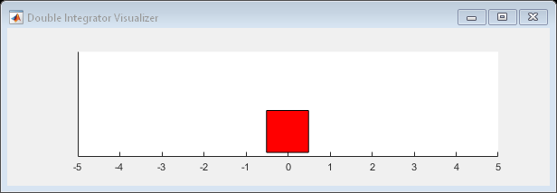
totalReward = sum(experience.Reward)
totalReward = -39.9140
References
[1] Sutton, Richard S., and Andrew G. Barto. Reinforcement Learning: An Introduction. Second edition. Adaptive Computation and Machine Learning Series. Cambridge, MA: The MIT Press, 2018.
See Also
Apps
Functions
Objects
Related Examples
More About
You can also select a web site from the following list:
Americas
- América Latina (Español)
- Canada (English)
- United States (English)
Europe
- Belgium (English)
- Denmark (English)
- Deutschland (Deutsch)
- España (Español)
- Finland (English)
- France (Français)
- Ireland (English)
- Italia (Italiano)
- Luxembourg (English)
- Netherlands (English)
- Norway (English)
- Österreich (Deutsch)
- Portugal (English)
- Sweden (English)
- Switzerland
- United Kingdom (English)