Train Reinforcement Learning Policy Using Custom Training Loop

This example shows how to define a custom training loop for a reinforcement learning policy. You can use this workflow to train reinforcement learning policies with your own custom training algorithms rather than using one of the built-in agents from the Reinforcement Learning Toolbox™ software.

Using this workflow, you can train policies that use any of the following policy and value function approximators.

• rlValueFunction - State value function approximator

• rlQValueFunction - State-action value function approximator with scalar output

• rlVectorQValueFunction - State-action function approximator with vector output

• rlContinuousDeterministicActor - Continuous deterministic actor

• rlDiscreteCategoricalActor - Discrete stochastic actor

• rlContinuousGaussianActor - Continuous Gaussian actor (stochastic)

In this example, a discrete actor policy with a discrete action space is trained using the REINFORCE algorithm (with no baseline). For more information on the REINFORCE algorithm, see Policy Gradient (PG) Agents.

Fix the random generator seed for reproducibility.

rng(0)

For more information on the functions you can use for custom training, see Functions for Custom Training.

Environment

For this example, a reinforcement learning policy is trained in a discrete cart-pole environment. The objective in this environment is to balance the pole by applying forces (actions) on the cart. Create the environment using the rlPredefinedEnv function.

env = rlPredefinedEnv("CartPole-Discrete");

Extract the observation and action specifications from the environment.

obsInfo = getObservationInfo(env);
actInfo = getActionInfo(env);

Obtain the dimension of the observation space (numObs) and the number of possible actions (numAct).

numObs = obsInfo.Dimension(1);
numAct = actInfo.Dimension(1);

For more information on this environment, see Load Predefined Control System Environments.

Policy

The reinforcement learning policy in this example is a discrete-action stochastic policy. It is modeled by a deep neural network that contains fullyConnectedLayer, reluLayer, and softmaxLayer layers. This network outputs probabilities for each discrete action given the current observations. The softmaxLayer ensures that the actor outputs probability values in the range [0 1] and that all probabilities sum to 1.

Create the deep neural network for the actor.

actorNetwork = [
    featureInputLayer(numObs)
    fullyConnectedLayer(24)
    reluLayer
    fullyConnectedLayer(24)
    reluLayer
    fullyConnectedLayer(2)
    softmaxLayer
    ];

Convert to dlnetwork. For more information, see dlaccelerate.

actorNetwork = dlnetwork(actorNetwork);

Create the actor using an rlDiscreteCategoricalActor object.

actor = rlDiscreteCategoricalActor(actorNetwork,obsInfo,actInfo);

Accelerate the gradient computation of the actor.

actorGradFcn = dlaccelerate(@actorLossFunction);

Evaluate the policy with a random observation as input.

policyEvalOutCell = evaluate(actor,{rand(obsInfo.Dimension)});
policyEvalOut = policyEvalOutCell{1}

policyEvalOut = 2x1 single column vector

    0.4682
    0.5318

Create a noisy policy from the actor.

policy = rlStochasticActorPolicy(actor);

Create the optimizer using rlOptimizer and rlOptimizerOptions function.

optimOpt = rlOptimizerOptions(LearnRate=5e-3,GradientThreshold=1);
actorOptimizer = rlOptimizer(optimOpt);

Training Setup

Configure the training to use the following options:

• Set up the training to last at most 5000 episodes, with each episode lasting at most 250 steps.

• To calculate the discounted reward, choose a discount factor of 0.995.

• Terminate the training after the maximum number of episodes is reached or when the average reward across 100 episodes reaches the value of 220.

numEpisodes = 5000;
maxStepsPerEpisode = 250;
discountFactor = 0.995;
avgWindowSize = 100;
trainingTerminationValue = 220;

Create a vector to store the cumulative reward for each training episode.

episodeCumulativeRewardVector = [];

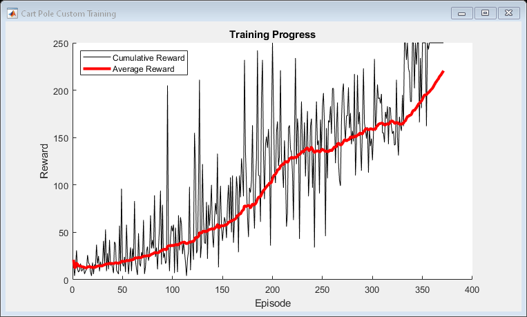
Create a figure for training visualization using the hBuildFigure helper function.

[trainingPlot,lineReward,lineAveReward] = hBuildFigure;

Custom Training Loop

The algorithm for the custom training loop is as follows. For each episode:

1. Create aggregated trajectory data buffers for storing experience information: observations, actions, and rewards.

2. Reset the environment.

3. Generate experiences until a terminal condition occurs. To do so, evaluate the policy to get actions, apply those actions to the environment, and obtain the resulting observations and rewards. Store the actions, observations, and rewards in buffers.

4. Compute the episode Monte Carlo return, which is the discounted future reward.

5. Compute the gradient of the loss function with respect to the policy parameters.

6. Update the actor using the computed gradients.

7. Update the training visualization.

8. Terminate training if the policy is sufficiently trained.

% Enable the training visualization plot.
set(trainingPlot,Visible="on");

% Create buffers for the training data, allocating enough data for 5
% full episodes. Learning will occur after each 5th episode finishes. 
% Aggregating multiple trajectories for on-policy learning can improve
% training convergence. Buffers are allocated as dlarrays to support
% automatic differentiation with 
% <docid:nnet_ref#mw_bdc503ca-68b1-4790-815e-6277f7d1e62e dlfeval> and 
% <docid:nnet_ref#mw_dc19e87d-b33c-4de3-8bec-3b7c6a37c3df dlgradient>.
trajectoriesForLearning = 5;
buffLen = trajectoriesForLearning*maxStepsPerEpisode;
observationBuffer = dlarray(zeros(numObs,1,buffLen));
% allocate valid actions for the action buffer
actionBuffer = dlarray(zeros(numAct,1,buffLen) + actInfo.Elements(1));
rewardBuffer = dlarray(zeros(1,buffLen));
returnBuffer = dlarray(zeros(1,buffLen));
% Create a "mask" variable to ensure that we are using consistent batch
% sizes for every gradient computation. The mask is used to "zero"
% advantages in the loss function for experiences beyond the actual
% number of steps taken in any given simulation. This ensures that
% additional accelerated functions are not generated for the actor loss
% function.
%
%     mask(i) == 1 for i <= batchSize
%     mask(i) == 0 for i >  batchSize
maskBuffer = dlarray(zeros(1,buffLen));
actionSet = repmat(actInfo.Elements',1,buffLen);

% Create a weighted discount matrix based on the max
% episode length. This will be used to compute the discountedReturn
% before learning.
v = 0:(maxStepsPerEpisode-1);
p = repmat(v',1,maxStepsPerEpisode) - v;
discountWeights = tril(discountFactor.^p);

% Train the policy for the maximum number of episodes 
% or until the average reward indicates that the policy 
% is sufficiently trained.
for episodeCt = 1:numEpisodes
    episodeOffset = ...
        mod(episodeCt-1,trajectoriesForLearning)*maxStepsPerEpisode;
    
    % 1. Reset the environment at the start of the episode
    obs = reset(env);    
    episodeReward = zeros(maxStepsPerEpisode,1);
    
    % 3. Generate experiences 
    %    for the maximum number of steps per episode 
    %    or until a terminal condition is reached.
    for stepCt = 1:maxStepsPerEpisode
        
        % Compute an action using the policy 
        % based on the current observation.
        action = getAction(policy,{obs});
        
        % Apply the action to the environment 
        % and obtain the resulting observation and reward.
        [nextObs,reward,isdone] = step(env,action{1});
        
        % Store the action, observation, 
        % and reward experiences in their buffers.
        j = episodeOffset + stepCt;
        observationBuffer(:,:,j) = obs;
        actionBuffer(:,:,j) = action{1};
        rewardBuffer(:,j) = reward;
        maskBuffer(:,j) = 1;
        
        obs = nextObs;
        
        % Stop if a terminal condition is reached.
        if isdone
            break;
        end
        
    end

    % Update the return buffer and cumulative reward for this episode.
    episodeElements = episodeOffset + (1:maxStepsPerEpisode);
    episodeCumulativeReward = extractdata(sum(rewardBuffer(episodeElements)));

    % 4. Compute the discounted future reward.
    returnBuffer(episodeElements) = rewardBuffer(episodeElements)*discountWeights;

    % Learn the set of aggregated trajectories.
    if mod(episodeCt,trajectoriesForLearning) == 0
        % Get the indices of each action taken in the action buffer.
        actionIndicationMatrix = dlarray(single(actionBuffer(:,:) == actionSet));

        % 5. Compute the gradient of the loss with respect to the actor
        % learnable parameters.
        actorGradient = dlfeval(actorGradFcn,...
            actor,{observationBuffer},actionIndicationMatrix,returnBuffer,maskBuffer);

        % 6. Update the actor using the computed gradients.
        [actor,actorOptimizer] = update( ...
            actorOptimizer, ...
            actor, ...
            actorGradient);

        % Update the policy from the actor
        policy = rlStochasticActorPolicy(actor);

        % flush the mask and reward buffer
        maskBuffer(:) = 0;
        rewardBuffer(:) = 0;
    end
    

    % 7. Update the training visualization.
    episodeCumulativeRewardVector = cat(2,...
        episodeCumulativeRewardVector,episodeCumulativeReward);
    movingAvgReward = movmean(episodeCumulativeRewardVector,...
        avgWindowSize,2);
    addpoints(lineReward,episodeCt,episodeCumulativeReward);
    addpoints(lineAveReward,episodeCt,movingAvgReward(end));
    drawnow;
    
    % 8. Terminate training if the network is sufficiently trained.
    if max(movingAvgReward) > trainingTerminationValue
        break
    end
    
end

Simulation

After training, simulate the trained policy.

Before simulation, reset the environment and set the policy to use the maximum likelihood (greedy) action.

obs = reset(env);
policy.UseMaxLikelihoodAction = true;

Enable the environment visualization, which is updated each time the environment step function is called.

plot(env)

For each simulation step, perform the following actions.

1. Get the action by sampling from the policy using the getAction function.

2. Step the environment using the obtained action value.

3. Terminate if a terminal condition is reached.

for stepCt = 1:maxStepsPerEpisode
    
    % Select action according to trained policy
    action = getAction(policy,{obs});
        
    % Step the environment
    [nextObs,reward,isdone] = step(env,action{1});
    
    % Check for terminal condition
    if isdone
        break
    end
    
    obs = nextObs;
    
end

Functions for Custom Training

To obtain actions and value functions for given observations from Reinforcement Learning Toolbox policy and value function approximators, you can use the following functions. These functions can also be used in automatically differentiated functions with dlfeval, dlgradient, and dlaccelerate.

• getValue — Obtain the estimated state value or state-action value function.

• getAction — Obtain the action from an actor based on the current observation.

• getMaxQValue — Obtain the estimated maximum state-action value function for a discrete Q-value approximator.

If your policy or value function approximator is a recurrent neural network, that is, a neural network with at least one layer that has hidden state information, the preceding functions can return the current network state. You can use the following function syntaxes to get and set the state of your approximator.

• state = critic.State — Obtain the state of approximator critic.

• critic.State = state — Set the state of approximator critic.

You can get and set the learnable parameters of your approximator using the getLearnableParameters and setLearnableParameters function, respectively.

In addition to these functions, you can use the dlgradient, update, and syncParameters functions to set parameters and compute gradients for your policy and value function approximators.

syncParameters

The syncParameters function updates the learnable parameters of one policy or value function approximator based on those of another approximator. This function is useful for updating a target actor or critic approximator, as is done for DDPG agents. To synchronize parameters values between two approximators, use the following syntax.

newTargetApproximator = syncParameters(
   oldTargetApproximator, ...
   sourceApproximator, ...
   smoothFactor)

Here:

• oldTargetApproximator is a policy or value function approximator object with parameters ${\theta }_{\mathrm{old}}$.

• sourceApproximator is a policy or value function approximator object with the same structure as oldTargetRep, but with parameters ${\theta }_{\mathrm{source}}$.

• smoothFactor is a smoothing factor ($\tau$) for the update.

• newTargetApproximator has the same structure as oldRep, but its parameters are ${\theta }_{\mathrm{new}}=\tau {\theta }_{\mathrm{source}}+\left(1-\tau \right){\theta }_{\mathrm{old}}$.

For more information, at the MATLAB® command line, type help rl.function.AbstractFunction.syncParameters.

Loss Function

The loss function in the REINFORCE algorithm the product between the discounted reward and the logarithm of the probability distribution of the action (coming from the policy evaluation for a given observation), summed across all time steps. An additional entropy loss is added to improve exploration and reduce over-fitting during training.

function actorGradient = actorLossFunction(actor,observation,actionIndicationMatrix,discountedReturn,mask)

    % Compute the advantage and apply it to the actions taken by the policy.
    advantage = actionIndicationMatrix.*discountedReturn.*mask;

    % Evaluate the action probabilities. Set the UseForward name-value pair
    % to true to support cases where the actor has layers that define a
    % forward pass different than prediction (e.g. batch normalization or
    % dropout layers).
    out = evaluate(actor,observation,UseForward=true);
    actionProbabilities = out{1};

    % Clip any action probability values less than eps to eps.
    actionProbabilities(actionProbabilities < eps) = eps;

    % Compute the log of the action probabilities.
    actionLogProbabilities = log(actionProbabilities);
    
    % Compute the policy gradient loss.
    pgLoss = -sum(advantage.*actionLogProbabilities,"all");

    % Compute the entropy loss.
    entropyLoss = -sum(actionProbabilities.*actionLogProbabilities.*mask,"all");

    % Compute the gradient of loss with respect to the actor learnable
    % parameters.
    loss = (pgLoss + 1e-4*entropyLoss)/(sum(mask));
    actorGradient = dlgradient(loss,actor.Learnables);
end

Helper Function

The following helper function creates a figure for training visualization.

function [trainingPlt, lineRewd, lineAvgRwd] = hBuildFigure()
    plotRatio = 16/9;
    trainingPlt = figure(...
                Visible="off",...
                HandleVisibility="off", ...
                NumberTitle="off",...
                Name="Cart Pole Custom Training");

    trainingPlt.Position(3) = ...
         plotRatio * trainingPlt.Position(4);
    
    ax = gca(trainingPlt);
    
    lineRewd = animatedline(ax);
    lineAvgRwd = animatedline(ax,Color="r",LineWidth=3);
    xlabel(ax,"Episode");
    ylabel(ax,"Reward");
    legend(ax,"Cumulative Reward","Average Reward", ...
           Location="northwest")
    title(ax,"Training Progress");
end