MOS Interconnect and Crosstalk Using RFCKT Objects
This example shows how to build and simulate an RC tree circuit using the RF Toolbox™.
In "Asymptotic Waveform Evaluation for Timing Analysis" (IEEE Transactions on Computer-Aided Design, Vol., 9, No. 4, April 1990), Pillage and Rohrer presented and simulated an RC tree circuit that models signal integrity and crosstalk in low- to mid-frequency MOS circuit interconnect. This example confirms their simulations using RF Toolbox software.
Their circuit, reproduced in the following figure, consists of 11 resistors and 12 capacitors. In the paper, Pillage and Rohrer:
Apply a ramp voltage input
Compute transient responses
Plot the output voltages across two different capacitors,
C7andC12.
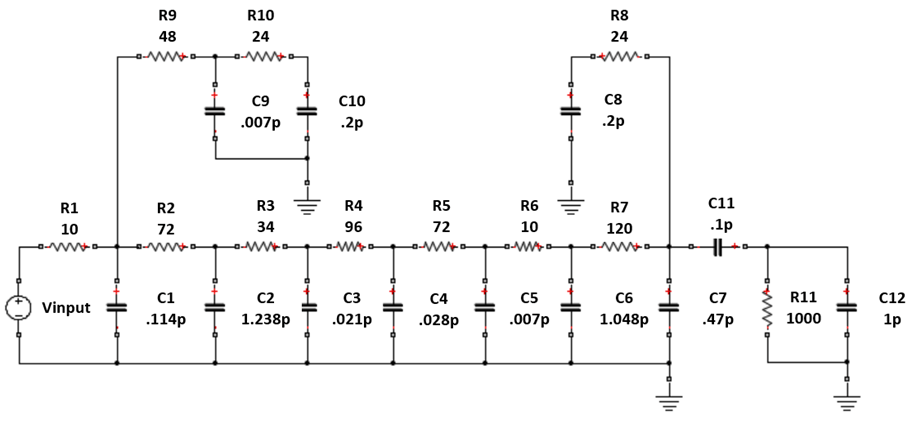
Figure 1: RC tree model of MOS interconnect with crosstalk.
With RF Toolbox software, you can programmatically construct this circuit in MATLAB® and perform signal integrity simulations.
This example shows:
How to use
rfckt.seriesrlc,rfckt.shuntrlc,rfckt.series, andrfckt.cascadeobject to programmatically construct the circuit as two different networks, depending on the desired output.How to use
analyzefunction to extract the S-parameters for each 2-port network over a wide frequency range.How to use
s2tffunction withZsource = 0andZload = Infto compute the voltage transfer function from input to each desired output.How to use
rationalfitfunction to produce rational-function approximations that capture the ideal RC-circuit behavior to a very high degree of accuracy.How to use
timerespfunction to compute the transient response to the input voltage waveform.
Redraw Circuit as Distinct 2-Port Networks
To duplicate both output plots, RF Toolbox calculates the output voltage across C7 and C12. To that end, the circuit must be expressed as two distinct 2-port networks, each with the appropriate capacitor at the output. Figure 2 shows the 2-port configuration for computing the voltage across C7. Figure 3 shows the configuration for C12. Both 2-port networks retain the original circuit topology, and share much of the same structure.
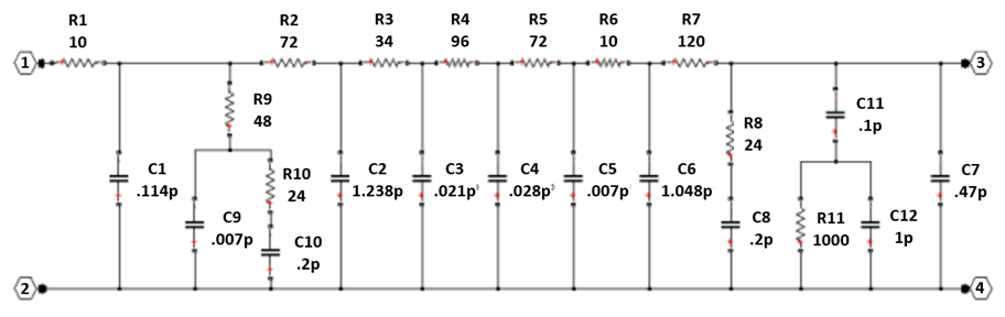
Figure 2: The circuit drawn as a 2-port network with output across C7.
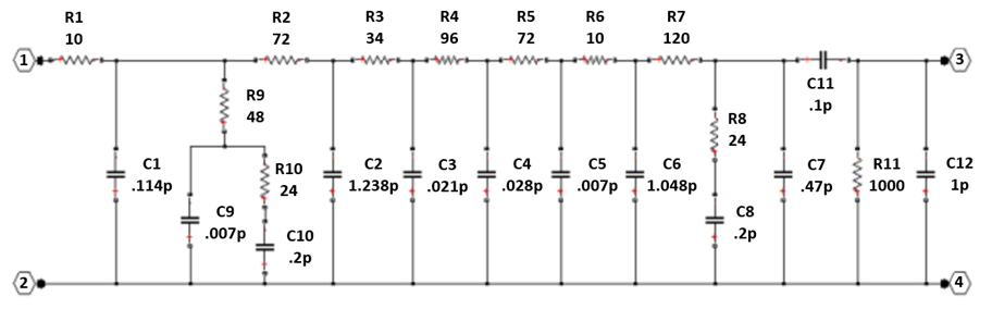
Figure 3: The circuit drawn as a 2-port network with output across C12.
Using RLC Building Blocks
All of the building blocks are formed by selecting appropriate values with the rfckt.shuntrlc object shown in Figure 4 or the rfckt.seriesrlc object shown in Figure 5. The 2-port building blocks are then connected using rfckt.cascade object as shown in Figure 6 or rfckt.series object as shown in Figure 7.
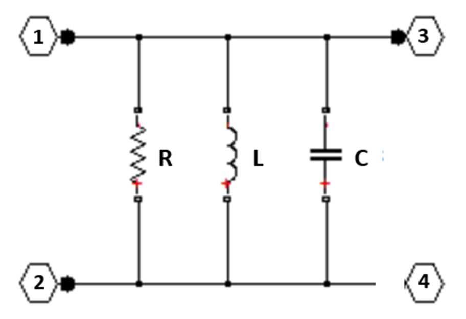
Figure 4: The 2-port network created using the rfckt.shuntrlc object.
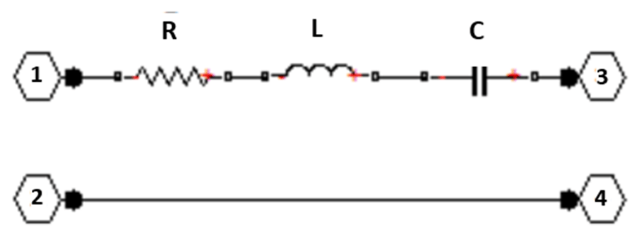
Figure 5: The 2-port network created using the rfckt.seriesrlc object.
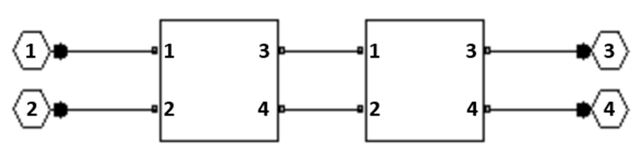
Figure 6: Connect 2-port networks with the rfckt.cascade object.
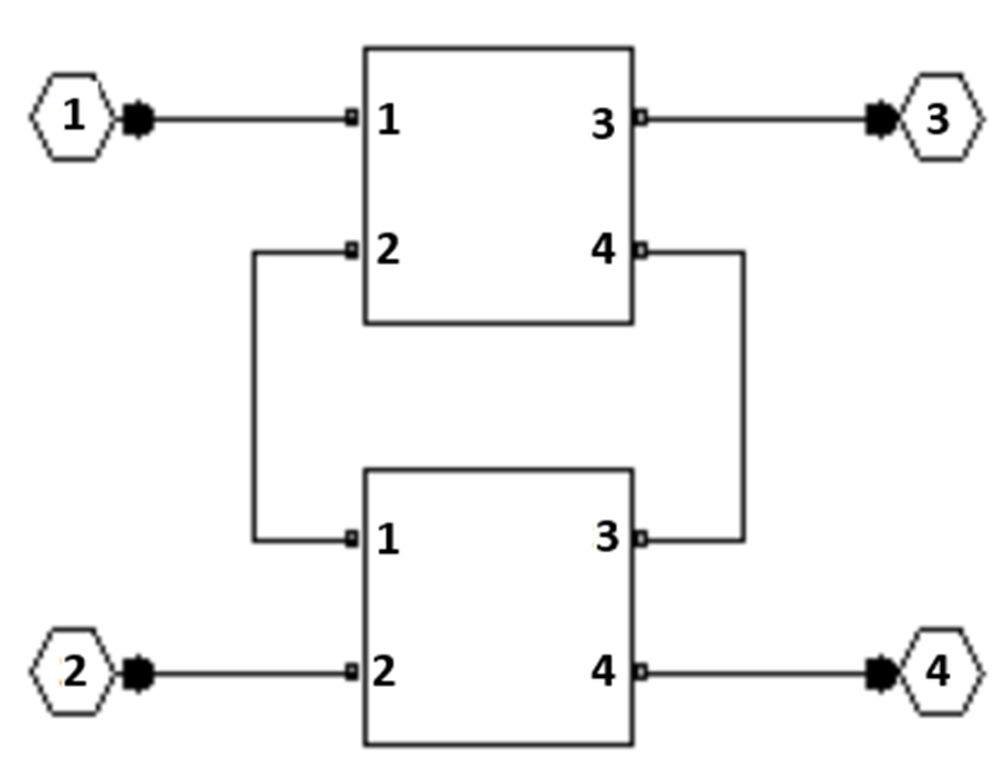
Figure 7: Connect 2-port networks with the rfckt.series object.
Shared Pieces of 2-Port Networks
The following MATLAB code constructs the portion of the network shared between the two variants.
R1 = rfckt.seriesrlc('R',10);
C1 = rfckt.shuntrlc('C',0.114e-12);
R9 = rfckt.shuntrlc('R',48);
C9 = rfckt.shuntrlc('C',0.007e-12);
R10 = rfckt.shuntrlc('R',24);
C10 = rfckt.shuntrlc('C',0.2e-12);
R10C10 = rfckt.series('Ckts',{R10,C10});
C9R10C10 = rfckt.cascade('Ckts',{C9,R10C10});
R9C9R10C10 = rfckt.series('Ckts',{R9,C9R10C10});
R2 = rfckt.seriesrlc('R',72);
C2 = rfckt.shuntrlc('C',1.238e-12);
R3 = rfckt.seriesrlc('R',34);
C3 = rfckt.shuntrlc('C',0.021e-12);
R4 = rfckt.seriesrlc('R',96);
C4 = rfckt.shuntrlc('C',0.028e-12);
R5 = rfckt.seriesrlc('R',72);
C5 = rfckt.shuntrlc('C',0.007e-12);
R6 = rfckt.seriesrlc('R',10);
C6 = rfckt.shuntrlc('C',1.048e-12);
R7 = rfckt.seriesrlc('R',120);
R8 = rfckt.shuntrlc('R',24);
C8 = rfckt.shuntrlc('C',0.2e-12);
R8C8 = rfckt.series('Ckts',{R8,C8});
sharedckt = rfckt.cascade('Ckts', ...
    {R1,C1,R9C9R10C10,R2,C2,R3,C3,R4,C4,R5,C5,R6,C6,R7,R8C8});

% Additional shared building blocks used in both 2-port networks.
C7 = rfckt.shuntrlc('C',0.47e-12);
R11C12 = rfckt.shuntrlc('R',1000,'C',1e-12);
Construct Each 2-Port Network
Figure 2 shows that constructing a 2-port network with an output port across C7 requires creating C11 using rfckt.shuntrlc object, then combining C11 with R11 and C12 using rfckt.series object, and finally combining C11R11C12 with the rest of the network and C7 using rfckt.cascade object.
Similarly, Figure 3 shows that constructing a 2-port network with an output port across C12 requires creating another version of C11 (C11b) using rfckt.seriesrlc object and combining all the parts together using rfckt.cascade object.
Construct shunt RLC circuit.
C11 = rfckt.shuntrlc('C',0.1e-12);
C11R11C12 = rfckt.series('Ckts',{C11,R11C12});
cktC7 = rfckt.cascade('Ckts',{sharedckt,C11R11C12,C7});
Construct series RLC circuit.
C11b = rfckt.seriesrlc('C',0.1e-12);
cktC12 = rfckt.cascade('Ckts',{sharedckt,C7,C11b,R11C12});
Simulation Setup
The input signal used by Pillage and Rohrer is a voltage ramp from 0 to 5 volts with a rise time of one nanosecond and a duration of ten nanoseconds. The following MATLAB code models this signal with 1000 timepoints with a sampleTime of 0.01 nanoseconds.
The following MATLAB code also uses the logspace function to generate a vector of 101 logarithmically spaced analysis frequencies between 1 Hz and 100 GHz. Specifying a wide set of frequency points improves simulation accuracy.
sampleTime = 1e-11;
t = (0:1000)'*sampleTime;
input = [(0:100)'*(5/100); (101:1000)'*0+5];
freq = logspace(0,11,101)';
Simulate Each 2-Port Network
To simulate each network:
The
analyzefunction extracts S-parameters over the specified frequency range.The
s2tffunction, withoption = 2, computes the gain from the source voltage to the output voltage. It allows arbitrary source and load impedances, in this caseZsource = 0andZload = Inf. The resulting transfer functionstfC7andtfC12are frequency-dependent data vectors that can be fit with rational-function approximation.The
rationalfitfunction generates high-accuracy rational-function approximations. The resulting approximations match the networks to machine accuracy.The
timerespfunction computes the analytic solution to the state-space equations defined by a rational-function approximation. This methodology is fast enough to enable one to push a million bits through a channel.
Simulate cktC7 circuit.
analyze(cktC7,freq);
sparamsC7 = cktC7.AnalyzedResult.S_Parameters;
tfC7 = s2tf(sparamsC7,50,0,Inf,2);
fitC7 = rationalfit(freq,tfC7);
outputC7 = timeresp(fitC7,input,sampleTime);
Simulate cktC12 circuit.
analyze(cktC12,freq);
sparamsC12 = cktC12.AnalyzedResult.S_Parameters;
tfC12 = s2tf(sparamsC12,50,0,Inf,2);
fitC12 = rationalfit(freq,tfC12);
outputC12 = timeresp(fitC12,input,sampleTime);
Plot Transient Responses
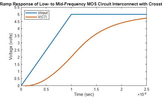
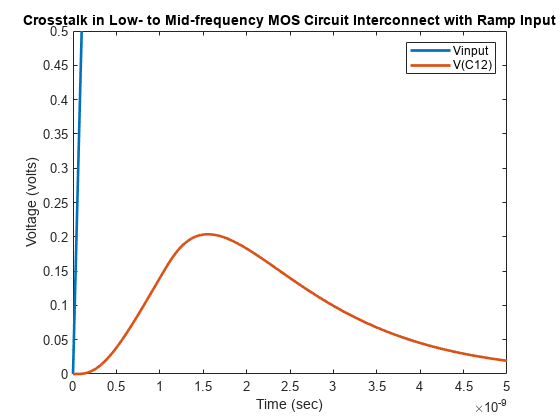
The outputs match Figures 23 and 24 of the Pillage and Rohrer paper. Plot the ramp response of low- to mid-frequency MOS circuit interconnect with crosstalk.
figure
plot(t,input,t,outputC7,'LineWidth',2)
axis([0 2.5e-9 0 5.5]);
title("Ramp Response of Low- to Mid-Frequency MOS Circuit Interconnect with Crosstalk");
xlabel("Time (sec)");
ylabel("Voltage (volts)");
legend("Vinput","V(C7)",Location="NorthWest");
Plot the crosstalk in low- to mid-frequency MOS circuit interconnect with ramp input.
figure
plot(t,input,t,outputC12,'LineWidth',2)
axis([0 5e-9 0 .5]);
title("Crosstalk in Low- to Mid-frequency MOS Circuit Interconnect with Ramp Input");
xlabel("Time (sec)");
ylabel("Voltage (volts)");
legend("Vinput","V(C12)",Location="NorthEast");
Verify Rational Fit Outside Fit Range
Though not shown in this example, you can also use the freqresp function to check the behavior of rationalfit function well outside the specified frequency range. The fit outside the specified range can sometimes cause surprising behavior, especially if frequency data near 0 Hz (DC) was not provided.
To perform this check for the rational-function approximation in this example, uncomment and run the following MATLAB code.
% widerFreqs = logspace(0,12,1001);
% respC7 = freqresp(fitC7,widerFreqs);
% figure
% loglog(freqs,abs(tfC7),'+',widerFreqs,abs(respC7))
% respC12 = freqresp(fitC12,widerFreqs);
% figure
% loglog(freqs,abs(tfC12),'+',widerFreqs,abs(respC12))