Control Manipulator Robot with Co-Simulation in Simulink and Gazebo
Simulate control of a robotic manipulator using co-simulation between Simulink and Gazebo. The example uses Simulink™ to model the robot behavior, generate control commands, send these commands to Gazebo, and control the pace of the Gazebo simulation.
The Gazebo Pacer block steps the Gazebo simulation at the same rate as Simulink, which enables commands to be executed accurately while simulating the physical dynamics in Gazebo.
The Gazebo Read and Gazebo Apply Command blocks are used for communication between MATLAB® and Gazebo.
The
gzlink,gzjoint, andgzworldfunctions provide easy access to model parameters and queries.
This example reviews each of these components and their configurations in detail using a Simulink model that controls the positions of a Universal Robotics UR10 manipulator. The model uses inverse kinematics to relate desired end effector pose to joint positions, then applies a joint-space PD controller with dynamic compensation feedforward terms to govern the motion.
For more information about setting up the environment for this example, see Configure Gazebo and Simulink for Co-simulation of a Manipulator Robot.
Set Up Gazebo with Robot Model and Plugin
To setup the Gazebo world, install the necessary plugins, and test the connection with MATLAB and simulink, see the Set Up Gazebo with Robot Model and Plugin section of the Configure Gazebo and Simulink for Co-simulation of a Manipulator Robot example.
Open World in Gazebo
Open the world by running these commands in the terminal of the Gazebo machine:
cd /home/user/src/GazeboPlugin/export
export SVGA_VGPU10=0
gazebo /home/user/worlds/Ur10BasicWithPlugin.world --verbose
Gazebo shows the robot and any other objects in the world. If the Gazebo simulator fails to open, you may need to reinstall the plugin. See Install Gazebo Plugin Manually in Perform Co-Simulation Between Simulink and Gazebo.

Connect to Gazebo
Next, initialize the Gazebo connection to MATLAB and Simulink. Specify the IP address and a port number of 14581, which is the default port for the Gazebo plugin.
ipGazebo = '192.168.116.162'; % Replace this with the IP of the Gazebo machine
gzinit(ipGazebo,14581);
Load the Robot Model
This model uses a universal UR10 robot created using loadrobot. The Gazebo model and robot models match since they are from the same source repository. For more information, see Configure Gazebo and Simulink for Co-simulation of a Manipulator Robot.
robot = loadrobot('universalUR10','Gravity',[0 0 -9.81],'DataFormat','column');
showdetails(robot)
--------------------
Robot: (10 bodies)

 Idx             Body Name                            Joint Name                            Joint Type             Parent Name(Idx)   Children Name(s)
 ---             ---------                            ----------                            ----------             ----------------   ----------------
   1             base_link                           world_joint                                 fixed                     world(0)   base(2)  shoulder_link(3)
   2                  base            base_link-base_fixed_joint                                 fixed                 base_link(1)
   3         shoulder_link                    shoulder_pan_joint                              revolute                 base_link(1)   upper_arm_link(4)
   4        upper_arm_link                   shoulder_lift_joint                              revolute             shoulder_link(3)   forearm_link(5)
   5          forearm_link                           elbow_joint                              revolute            upper_arm_link(4)   wrist_1_link(6)
   6          wrist_1_link                         wrist_1_joint                              revolute              forearm_link(5)   wrist_2_link(7)
   7          wrist_2_link                         wrist_2_joint                              revolute              wrist_1_link(6)   wrist_3_link(8)
   8          wrist_3_link                         wrist_3_joint                              revolute              wrist_2_link(7)   ee_link(9)  tool0(10)
   9               ee_link                        ee_fixed_joint                                 fixed              wrist_3_link(8)
  10                 tool0        wrist_3_link-tool0_fixed_joint                                 fixed              wrist_3_link(8)
--------------------
Set the initial configuration of the robot.
q0 = [0 -70 140 0 0 0]' * pi/180;
Load Simulink Model
The gazeboCosimControl model controls the end-effector position of the manipulator using the sliders in the User Input: End Effector section. The Inverse Kinematics subsystem generates a joint configuration that achieves the desired position. Then, the Joint Controller subsystems generates torque forces for each joint to reach this position
Open the model.
open_system('gazeboCosimControl');
Set Controller and Trajectory Sample Times
Ts = 0.01;
Ts_trajectory = 0.05;
The sample time of the controller is short to ensure good performance. The sample time of trajectory is longer to ensure simulation speed, which is typical for high-level tasks like camera sensor, inverse kinematics, and trajectory generation.
Understand the model construction
The Simulink model consists of four areas:
User input: Provides inputs for the desired robot end effector position using sliders.
Control: Maps the end effector position to joint position using inverse kinematics and controls joint position using a computed torque controller
Gazebo Pacer: Maintains the connection to Gazebo to ensure that the Simulink model steps both simulations.
Gazebo Robot: Sends commands to and receives commands from the Gazebo world.
These sections are outlined in greater detail below.
User Input
The user input has 6 sliders that control the end effector position: three to control the X, Y, and Z position in space, and three to control the orientation.
Control

The control section translates the desired end-effector pose to joint torques. First, the Inverse Kinematics subsystem computes joint positions that satisfy a target end-effector pose. Next, the Joint Controller subsystem produces actuator input torques given the joint reference position, velocity, and acceleration, and the current robot state. The state contains the measured position and velocity output from Gazebo.
Inverse Kinematics Subsystem
Inverse kinematics calculates the joint position for the corresponding end effector pose (position and orientation) given an initial guess. For fast convergence, set the initial condition of the unit delay. In this subsystem, the weights are uniform, implying that the solution should place equal importance on achieving all positions and orientations in the desired pose.

Joint Controller subsystem
In this example, the joint controller uses feedback and a feedforward terms. Gravity torque and velocity product values combine to form the feedforward term. A proportional-derivative (PD) controller generates the feedback term. For more details about joint controllers, refer to Perform Safe Trajectory Tracking Control Using Robotics Manipulator Blocks.

Gazebo Pacer
The Gazebo Pacer block ensures co-simulation with Gazebo by stepping the Gazebo simulation in sync with Simulink steps. This is important for applications like this model, where a controller is used to directly govern the position of a robot in the Gazebo world. The joint measurements and torque commands must be synced to ensure the simulation reflects of the actual behavior.
In the block mask, specify the sample time as Ts. You can test your Gazebo connection using the Configure Gazebo network and simulation settings link. This connection was already set up using gzinit.

Gazebo Model
The Gazebo Model subsystem contains the blocks used to communicate with the Gazebo world. In this case, the controller applies a torque to each joint and reads back the joint position and velocity.

Apply Joint Torque
For each joint, the torque must be applied in the Set <joint name> subsystems of the Transmit to Gazebo area of the Gazebo model subsystem. For example, for the shoulder pan joint, the tools to send the shoulder plan subsystem are contained in the Set Shoulder Pan subsystem.

Each of these subsystems uses a Bus Assignment block whose inputs define the type of bus, the details of the model and duration, and the resultant command.
The Gazebo Blank Message block defines the bus type to be a Gazebo message format of the appropriate type. In the block parameters dialog, select "ApplyJointTorque" from the list of command types. The block is required to ensure that the correct bus template is used, i.e. that the port is the Bus Assignment block have the correct values. 
The Gazebo Select Entity block selects the object to which this message will be applied. In this case, since a torque is being applied, the "entity" is a joint. Since this subsystem will apply torque to the shoulder joint, select the corresponding joint in the Gazebo world from the list of entity types. As long as a connection to the Gazebo world has been established, this list will be automatically populated. If the connection is lost, click the "Configure Gazebo network and simulation settings" link to reestablish, or use the gzinit command line interface. The Gazebo world must be open for this operation to succeed.

The Gazebo Apply Command block takes the contents of the message sends it to the Gazebo server. Open the block dialog parameters, select the Command type parameter, and select ApplyJointTorque to send the corresponding command to Gazebo.

The remaining inputs govern the amount and duration of the applied force. The effort inport specifies the joint torque quantity. The index input dictates the axis to which the torque should be applied. Since each of the revolute joints is just 1 degree of freedom, this value should be set to uint32(0) to indicate the first axis. Finally, the duration inputs specify the duration of the applied torque, divided into seconds and nanoseconds. For example, if a duration is 1.005 seconds, it would be 1 second and 5,000,000 nanoseconds as a bus. They are separated out to increase precision. In this case, the controller applies the torque for the length of the sample time, previously specified to 0.01 seconds, or 1e7 nanoseconds. Therefore the first input is zero (0 seconds) and the second input is 1e7.

The Gazebo Model subsystem includes 5 other subsystems corresponding to the other five joints, which have been configured in the same fashion.
Measure Joint State
The second part of the Gazebo Model interface requires reading values from Gazebo using the Gazebo Read block for each joint. For example, the block for the shoulder pan joint is shown below.

The Gazebo Read block reads messages from the Gazebo server. In the block dialog, click "Select.." next to the topic to choose the right topic to read from, and select the corresponding measured joint value, /gazebo/ground_truth/joint_state/ur10/shoulder_pan_joint. This message selects the precise ground truth value, though it is also possible to place sensors in Gazebo and read from those instead.
Use the Bus Selector to only choose the relevant values from the message. In this case, only the position is measured from the Gazebo model, which is ultimately fed back to the controller.
This section also reads back the value of the red box in Gazebo. While it is possible to also set the position of this box using a format similar to that used above, it is simpler to use the gzlink command line interface to update the block at discrete instants during the model execution.
Customize Bus Objects for Simulation
Gazebo bus objects are generated when the cosimulation blocks are introduced in a model. Signals from Gazebo are read through these bus objects. By default, dimensions are set to variable size since joints can have multiple degrees of freedom. Since all joints in this example are revolute joints, they are 1-dimensional and fixed in size, which can be specified as a property of the bus signals**.** This step is optional, but it is useful to overcome limitations of variable-size signals.
Load the custom bus objects.
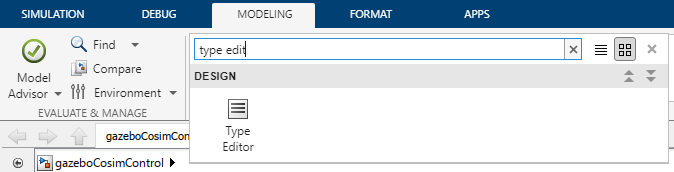
load('custom_busobjects_basic'); To interactively load the bus objects, open the Type Editor in Simulink. In the Simulink Toolstrip, on the Modeling tab, in the Design gallery, click Type Editor.
In the Type Editor, select the base workspace as the destination for the import. Then, click the ![]() button arrow and select MAT File.
button arrow and select MAT File.

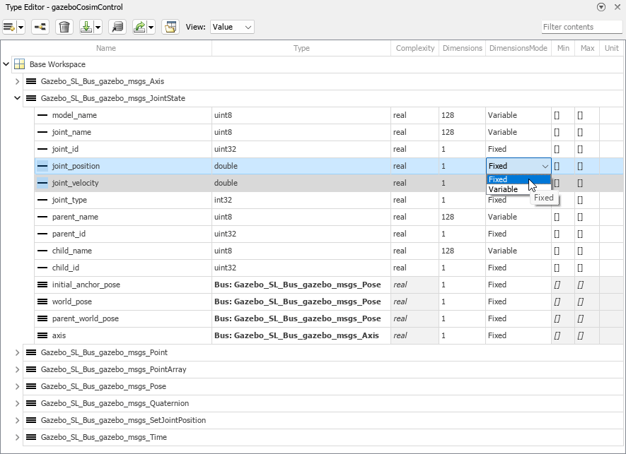
In the dialog box that opens, select the MAT file to load. To view the properties of the loaded bus objects, set View to Value.
In the Type Editor table, select the bus object used to read joint state, then select the corresponding element name. For the bus object named Gazebo_SL_Bus_gazebo_msgs_JointState, select the elements named joint_position and joint_velocity and change Dimension to 1 and DimensionMode to Fixed.
Run the Simulation
Reset the Gazebo world and box position before simulating using MATLAB commands. Commands like these can be more directly incorporated into the Simulink model as a StartFcn callback to ensure that they are executed at each Simulation run. In the Gazebo Pacer block parameters, only the simulation time is reset when you run the model unless you change the Reset Behavior drop down.
gzworld("reset"); % Reset the world to its initial state
gzlink("set","redBox","link","Position",[0.5 -0.4 .3]); % Move the box to a new location
STATUS:  Succeed


MESSAGE:  Parameter set successfully.
You can also run these types of commands during simulation. To do so, click run to simulate the Simulink model rather than the sim command to ensure that the command line can be executed while the simulation is running.
Run the simulation for 20 seconds and test different poses using the sliders in User Input: End Effector. Verify the inverse kinematics and joint controller are behaving properly in Gazebo.
simoutput = sim('gazeboCosimControl','StopTime','20');

Use the Simulation Data Inspector to see behavior of the joint positions. This image shows data when the manipulator command positions have been changed several times over the course of the simulation.

View Performance
Joint measurements and references are logged. Once the simulation is complete, plot the logged outputs.
measuredPosition = simoutput.logsout{1}.Values;
referencePosition = simoutput.logsout{2}.Values;
figure
plot(measuredPosition.Time, measuredPosition.Data, '-', referencePosition.Time, referencePosition.Data, '--')
legend({'Meas1','Meas2','Meas3','Meas4','Meas5','Meas6','Ref1','Ref2','Ref3','Ref4','Ref5','Ref6'})