Path Following for a Differential Drive Robot
This example demonstrates how to control a robot to follow a desired path using a Robot Simulator. The example uses the Pure Pursuit path following controller to drive a simulated robot along a predetermined path. A desired path is a set of waypoints defined explicitly or computed using a path planner (refer to Path Planning in Environments of Different Complexity). The Pure Pursuit path following controller for a simulated differential drive robot is created and computes the control commands to follow a given path. The computed control commands are used to drive the simulated robot along the desired trajectory to follow the desired path based on the Pure Pursuit controller.
Define Waypoints
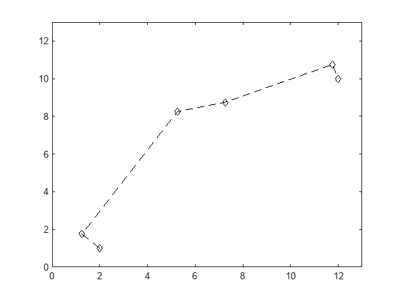
Define a set of waypoints for the desired path for the robot.
path = [2.00 1.00;
        1.25 1.75;
        5.25 8.25;
        7.25 8.75;
        11.75 10.75;
        12.00 10.00];
Set the current location and the goal location of the robot as defined by the path.
robotInitialLocation = path(1,:);
robotGoal = path(end,:);
Assume an initial robot orientation (the robot orientation is the angle between the robot heading and the positive x-axis, measured counterclockwise).
initialOrientation = 0;
Define the current pose for the robot [x y theta].
robotCurrentPose = [robotInitialLocation initialOrientation]';
Create a Kinematic Robot Model
Initialize the robot model and assign an initial pose. The simulated robot has kinematic equations for the motion of a two-wheeled differential drive robot. The inputs to this simulated robot are linear and angular velocities.
robot = differentialDriveKinematics(TrackWidth=1,VehicleInputs="VehicleSpeedHeadingRate");Visualize the desired path.
figure
plot(path(:,1),path(:,2),"-*")
title("Desired Path")
xlabel("X")
ylabel("Y")
axis padded
Define the Path Following Controller
Based on the path defined above and a robot motion model, you need a path following controller to drive the robot along the path. Create the path following controller using the controllerPurePursuit object.
controller = controllerPurePursuit;
Use the path defined above to set the desired waypoints for the controller.
controller.Waypoints = path;
Set the path following controller parameters. The desired linear velocity is set to 0.6 meters/second for this example.
controller.DesiredLinearVelocity = 0.6;
The maximum angular velocity acts as a saturation limit for rotational velocity, which is set at 2 radians/second for this example.
controller.MaxAngularVelocity = 2;
As a general rule, the look-ahead distance should be larger than the desired linear velocity for a smooth path. The robot might cut corners when the look-ahead distance is large. In contrast, a small look-ahead distance can result in an unstable path following behavior. A value of 0.3 m was chosen for this example.
controller.LookaheadDistance = 0.3;
Use Path Following Controller to Drive the Robot Over Desired Waypoints
The path following controller provides input control signals for the robot, which the robot uses to drive itself along the desired path.
Define a goal radius, which is the desired distance threshold between the robot's final location and the goal location. Once the robot is within this distance from the goal, it will stop. Also, you compute the current distance between the robot location and the goal location. This distance is continuously checked against the goal radius and the robot stops when this distance is less than the goal radius.
Note that too small value of the goal radius may cause the robot to miss the goal, which may result in an unexpected behavior near the goal.
goalRadius = 0.1;
distanceToGoal = norm(robotInitialLocation - robotGoal);
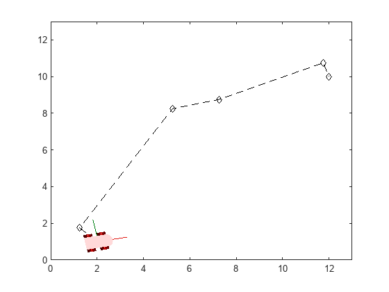
The controllerPurePursuit object computes control commands for the robot. Drive the robot using these control commands until it reaches within the goal radius. If you are using an external simulator or a physical robot, then the controller outputs should be applied to the robot and a localization system may be required to update the pose of the robot. The controller runs at 10 Hz.
% Initialize the simulation loop
sampleTime = 0.1;
vizRate = rateControl(1/sampleTime);

% Initialize the figure
figure

% Determine vehicle frame size to most closely represent vehicle with plotTransforms
frameSize = robot.TrackWidth/0.8;

while(distanceToGoal > goalRadius)

    % Compute the controller outputs, i.e., the inputs to the robot
    [v,omega] = controller(robotCurrentPose);

    % Get the robot's velocity using controller inputs
    vel = derivative(robot,robotCurrentPose,[v omega]);

    % Update the current pose
    robotCurrentPose = robotCurrentPose + vel*sampleTime;

    % Re-compute the distance to the goal
    distanceToGoal = norm(robotCurrentPose(1:2) - robotGoal(:));

    % Update the plot
    hold off

    % Plot path each instance so that it stays persistent while robot mesh
    % moves
    plot(path(:,1),path(:,2),"-*")
    title("Animation of Robot Following Path")
    hold on

    % Plot the path of the robot as a set of transforms
    plotTrVec = [robotCurrentPose(1:2); 0];
    plotRot = axang2quat([0 0 1 robotCurrentPose(3)]);
    plotTransforms(plotTrVec',plotRot, ...
        MeshFilePath="groundvehicle.stl",Parent=gca,View="2D",FrameSize=frameSize);
    xlim([0 13])
    ylim([0 13])

    waitfor(vizRate);
end
Using the Path Following Controller Along with PRM
If the desired set of waypoints are computed by a path planner, the path following controller can be used in the same fashion. First, visualize the map.
load exampleMaps
map = binaryOccupancyMap(simpleMap);
figure
show(map)![Figure contains an axes object. The axes object with title Binary Occupancy Grid, xlabel X [meters], ylabel Y [meters] contains an object of type image.](../../examples/robotics/win64/PathFollowingControllerExample_03.png)
You can compute the path using the PRM path planning algorithm. See Path Planning in Environments of Different Complexity for details.
mapInflated = copy(map);
inflate(mapInflated,robot.TrackWidth/2);
prm = robotics.PRM(mapInflated);
prm.NumNodes = 100;
prm.ConnectionDistance = 10;
Find a path between the start and end location. Note that the path will be different due to the probabilistic nature of the PRM algorithm.
startLocation = [4.0 2.0];
endLocation = [24.0 20.0];
path = findpath(prm,startLocation,endLocation)
path = 8×2

     4.0000     2.0000
     3.1703     2.7616
     7.0797    11.2229
     8.1337    13.4835
    14.0707    17.3248
    16.8068    18.7834
    24.4564    20.6514
    24.0000    20.0000
Display the inflated map, the road maps, and the final path.
show(prm);
![Figure contains an axes object. The axes object with title Probabilistic Roadmap, xlabel X [meters], ylabel Y [meters] contains 4 objects of type image, line, scatter.](../../examples/robotics/win64/PathFollowingControllerExample_04.png)
You defined a path following controller above which you can re-use for computing the control commands of a robot on this map. To re-use the controller and redefine the waypoints while keeping the other information the same, use the release function.
release(controller);
controller.Waypoints = path;
Set initial location and the goal of the robot as defined by the path.
robotInitialLocation = path(1,:);
robotGoal = path(end,:);
Assume an initial robot orientation.
initialOrientation = 0;
Define the current pose for robot motion [x y theta].
robotCurrentPose = [robotInitialLocation initialOrientation]';
Compute distance to the goal location.
distanceToGoal = norm(robotInitialLocation - robotGoal);
Define a goal radius.
goalRadius = 0.1;
Drive the robot using the controller output on the given map until it reaches the goal. The controller runs at 10 Hz.
reset(vizRate);

% Initialize the figure
figure

while(distanceToGoal > goalRadius)

    % Compute the controller outputs, i.e., the inputs to the robot
    [v,omega] = controller(robotCurrentPose);

    % Get the robot's velocity using controller inputs
    vel = derivative(robot,robotCurrentPose,[v omega]);

    % Update the current pose
    robotCurrentPose = robotCurrentPose + vel*sampleTime;

    % Re-compute the distance to the goal
    distanceToGoal = norm(robotCurrentPose(1:2) - robotGoal(:));

    % Update the plot
    hold off
    show(map);
    hold on

    % Plot path each instance so that it stays persistent while robot mesh
    % moves
    plot(path(:,1),path(:,2),"-*")

    % Plot the path of the robot as a set of transforms
    plotTrVec = [robotCurrentPose(1:2); 0];
    plotRot = axang2quat([0 0 1 robotCurrentPose(3)]);
    plotTransforms(plotTrVec',plotRot,MeshFilePath="groundvehicle.stl",Parent=gca,View="2D",FrameSize=frameSize);
    light;
    xlim([0 27])
    ylim([0 26])

    waitfor(vizRate);
end
![Figure contains an axes object. The axes object with title Binary Occupancy Grid, xlabel X [meters], ylabel Y [meters] contains 6 objects of type patch, line, image.](../../examples/robotics/win64/PathFollowingControllerExample_05.png)