ncfsyn

Loop shaping design using Glover-McFarlane method

Syntax

[K,CL,gamma,info] = ncfsyn(G)

[K,CL,gamma,info] = ncfsyn(G,W1)

[K,CL,gamma,info] = ncfsyn(G,W1,W2)

[K,CL,gamma,info] = ncfsyn(G,W1,W2,tol)

Description

ncfsyn implements a method for designing controllers that uses a combination of loop shaping and robust stabilization as proposed in [1]-[2]. The function computes the Glover-McFarlane H_∞ normalized coprime factor loop-shaping controller K for a plant G with pre-compensator and post-compensator weights W₁ and W₂. The function assumes the positive feedback configuration of the following illustration.

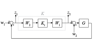
To specify negative feedback, replace G by –G. The controller K_s stabilizes a family of systems given by a ball of uncertainty in the normalized coprime factors of the shaped plant G_s = W₂GW₁. The final controller K returned by ncfsyn is obtained as K = W₁K_sW₂.

[K,CL,gamma,info] = ncfsyn(G) computes the Glover-McFarlane H_∞ normalized coprime factor loop-shaping controller K for the plant G, with W₁ = W₂ = I. CL is the closed-loop system from the disturbances w₁ and w₂ to the outputs z₁ and z₂. The function also returns the H_∞ performance gamma, and a structure containing additional information about the result.

[K,CL,gamma,info] = ncfsyn(G,W1) computes the controller using the pre-compensator weight you specify in W1, with W₂ = I.

[K,CL,gamma,info] = ncfsyn(G,W1,W2) computes the controller using the specified pre-compensator weight W1 and post-compensator weight W2.

[K,CL,gamma,info] = ncfsyn(G,W1,W2,tol) specifies how tightly the performance gamma of the synthesized controller approximates the optimal achievable performance gopt. Increasing tol can help when the controller K has undesirable fast dynamics.

Examples

Loop Shaping with ncfsyn

Use ncfsyn to design a controller for the following plant.

G = tf([1 5],[1 2 10]);

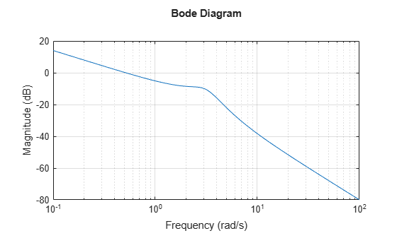
Use weighting functions that yield a shaped plant W1*G*W2 with high gain for disturbance attenuation below 0.1 rad/s, and low gain for good robust stability above about 5 rad/s. For this G, a pre-compensator weight alone is sufficient.

W1 = tf(1,[1 0]);
bodemag(W1*G)
grid

Compute the controller.

[K,CL,gamma,info] = ncfsyn(G,W1);

The optimal cost gamma is related to the normalized coprime stability margin of the system by 1/gamma = ncfmargin(Gs,-Ks). (The minus sign is needed because ncfmargin assumes a negative-feedback loop, while ncfsyn computes a positive-feedback controller.)

b = ncfmargin(info.Gs,-info.Ks);
[gamma 1/b]

ans = 1×2

    1.4521    1.4521

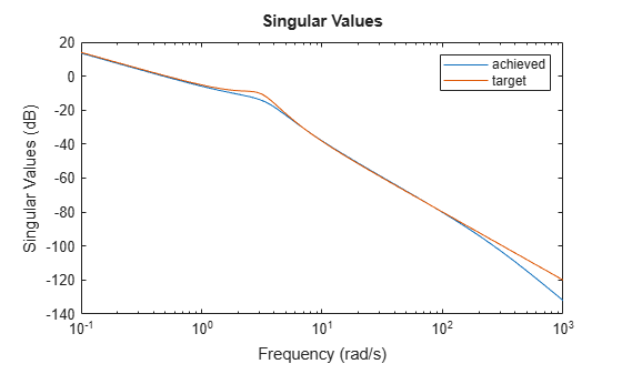
Compare the achieved and target loop shapes.

sigma(G*K,G*W1)
legend('achieved','target')

Reduce Undesirable Fast Dynamics in Controller

In the controller returned by ncfsyn, some controller poles can become infinitely fast as the actual performance gamma approaches the optimal achievable performance gopt. To prevent this, check the controller poles and increase the tol argument if some poles are undesirably fast. tol sets how closely gamma of the synthesized controller approximates gopt.

Load G, a fourth-order plant.

load("ncfsynTolPlant.mat")
bode(G)

Use a weighting function that yields a shaped plant W1*G with high gain for disturbance attenuation below about 10 rad/s, and low gain for good robust stability above about 1000 rad/s.

W1 = zpk(-130,0,0.6);
bode(W1*G)

Design a controller using the default tolerance, tol = 1e-3. Examine the poles of the resulting controller.

[K1,~,gamma1,info1] = ncfsyn(G,W1);
damp(K1)

                                                                       
         Pole              Damping       Frequency      Time Constant  
                                       (rad/seconds)      (seconds)    
                                                                       
  0.00e+00                -1.00e+00       0.00e+00              Inf    
 -1.48e+02 + 1.60e+01i     9.94e-01       1.49e+02         6.76e-03    
 -1.48e+02 - 1.60e+01i     9.94e-01       1.49e+02         6.76e-03    
 -7.90e+02 + 8.01e+02i     7.02e-01       1.13e+03         1.27e-03    
 -7.90e+02 - 8.01e+02i     7.02e-01       1.13e+03         1.27e-03    
 -1.50e+05                 1.00e+00       1.50e+05         6.66e-06    

This controller has a pole at around 150000 rad/s, much faster than any other dynamics in the controller. To reduce the frequency of this pole, try increasing the tolerance to 0.1.

tol = 0.1;
[K2,~,gamma2,info2] = ncfsyn(G,W1,[],tol);
damp(K2)

                                                                       
         Pole              Damping       Frequency      Time Constant  
                                       (rad/seconds)      (seconds)    
                                                                       
  0.00e+00                -1.00e+00       0.00e+00              Inf    
 -1.50e+02 + 6.85e+00i     9.99e-01       1.50e+02         6.68e-03    
 -1.50e+02 - 6.85e+00i     9.99e-01       1.50e+02         6.68e-03    
 -6.58e+02 + 9.45e+02i     5.71e-01       1.15e+03         1.52e-03    
 -6.58e+02 - 9.45e+02i     5.71e-01       1.15e+03         1.52e-03    
 -1.77e+03                 1.00e+00       1.77e+03         5.65e-04    

This time the highest-frequency pole is closer to the others. Compare the resulting performance values to confirm that the two controllers deliver similar performance.

gamma1, gamma2

gamma1 = 2.1157

gamma2 = 2.3250

Input Arguments

G — Plant

dynamic system model

Plant, specified as a dynamic system model such as a state-space (ss) model. If G is a generalized state-space model with uncertain or tunable control design blocks, then ncfsyn uses the nominal or current value of those elements.

W1 — Pre-compensator weight

eye(Nu) (default) | LTI model

Pre-compensator weight, specified as:

• Identity matrix eye(Nu), where Nu is the number of inputs in G.

• SISO minimum-phase LTI model. In this case, ncfsyn uses the same weight for every loop channel.

• MIMO minimum-phase LTI model with Nu inputs and outputs.

Select pre-compensator and post-compensator weights W1 and W2 such that the gain of the shaped plant G_s = W2*G*W1 is sufficiently high at frequencies where good disturbance attenuation is required, and sufficiently low at frequencies where good robust stability is required.

W2 — Post-compensator weight

eye(Ny) (default) | LTI model | []

Post-compensator weight, specified as:

• Identity matrix eye(Ny), where Ny is the number of outputs in G.

• SISO minimum-phase LTI model. In this case, ncfsyn uses the same weight for every loop channel.

• MIMO minimum-phase LTI model with Ny inputs and outputs.

• [], if you want to omit W2 while using the tol input argument. Setting W2 = [] is equivalent to setting W2 = eye(Ny).

Select pre-compensator and post-compensator weights W1 and W2 such that the gain of the shaped plant G_s = W2*G*W1 is sufficiently high at frequencies where good disturbance attenuation is required, and sufficiently low at frequencies where good robust stability is required.

tol — Near-optimality tolerance

0.001 (default) | positive scalar

Near-optimality tolerance, specified as a positive scalar value. ncfsyn returns a controller K with performance gamma that satisfies abs(gamma-gopt) < tol*gopt, where gopt is the optimal performance (returned in info). Use tol to adjust the acceptable gap between gamma and gopt. A tol value that is too small can cause numerical difficulties and introduce fast poles in K. Increasing tol usually eliminates both issues. For an example, see Reduce Undesirable Fast Dynamics in Controller.

Output Arguments

K — H_∞-optimal loop-shaping controller

state-space (ss) model

H_∞-optimal loop-shaping controller, returned as a state-space (ss) model with the same number of inputs as G has outputs and the same number of outputs as G has inputs. The optimal controller K = W₁K_sW₂. See Algorithms.

CL — Optimal closed-loop system

state-space (ss) model

Optimal closed-loop system from the disturbances w₁ and w₂ to the outputs z₁ and z₂, returned as a state-space model. The closed-loop system is given by:

$$\left[\begin{array}{c}I\\ K\end{array}\right]{\left(I-GK\right)}^{-1}\left[I,G\right].$$

gamma — H_∞ performance

positive scalar value

H_∞ performance achieved with the controller K, returned as a positive scalar value greater than 1. The H_∞ performance is hinfnorm(CL). The optimal controller K_s is such that the singular-value plot of the shaped loop L_s = W₂GW₁K_s optimally matches the target loop shape G_s to within a factor of gamma. However, for numerical reasons, ncfsyn generally returns a controller with slightly larger H_∞ performance than optimal. For the optimal achievable performance, see the info output argument.

gamma is related to the normalized coprime stability margin of the system by gamma = 1/ncfmargin(Gs,-Ks). Thus, gamma gives a good indication of robustness of stability to a wide class of unstructured plant variations, with values in the range 1 < gamma < 3 corresponding to satisfactory stability margins for most typical control system designs.

info — Additional information

structure

Additional information about the controller synthesis, returned as a structure containing the following fields.

• gopt — Optimal performance achievable by H_∞ synthesis for the shaped plant. For numerical reasons, ncfsyn generally returns a controller with slightly larger H_∞ performance, which is returned in gamma. To adjust how tightly ncfsyn aims to make gamma match gopt, use the tol input argument. See Reduce Undesirable Fast Dynamics in Controller.

• emax — nugap robustness metric, emax = 1/gopt (see gapmetric)

• Gs — Shaped plant G_s = W₂GW₁

• Ks — Optimal controller for shaped plant Gs. The final controller is K = W₁K_sW₂. See Algorithms for details.

Tips

• While ncfmargin assumes a negative-feedback loop, the ncfsyn command designs a controller for a positive-feedback loop. Therefore, to compute the margin using a controller designed with ncfsyn, use [marg,freq] = ncfmargin(G,K,+1).

Algorithms

The returned controller K = W₁K_sW₂, where K_s is an optimal H_∞ controller that minimizes the H_∞ cost

$$\gamma \left(K_s\right)={\Vert \left[\begin{array}{c}I\\ K_s\end{array}\right]{(I-G_s{K}_s)}^{-1}[I,G_s]\Vert }_{\infty }={\Vert \left[\begin{array}{c}I\\ G_s\end{array}\right]{(I-K_s{G}_s)}^{-1}[I,K_s]\Vert }_{\infty }.$$

The optimal performance is the minimal cost

$$\gamma :=\underset{K_s}{\min }\gamma \left(K_s\right).$$

Suppose that G_s=NM^–1, where N(jω)*N(jω) + M(jω)*M(jω) = I, is a normalized coprime factorization (NCF) of the weighted plant model G_s. Then, theory ensures that the control system remains robustly stable for any perturbation $${\tilde{G}}_s$$ to G_s of the form

$${\tilde{G}}_s=(N+{\Delta }_1){(M+{\Delta }_2)}^{-1}$$

where Δ₁, Δ₂ are a stable pair satisfying

$${\Vert \left[\begin{array}{c}{\Delta }_1\\ {\Delta }_2\end{array}\right]\Vert }_{\infty }<MARG:=\frac{1}{\gamma }.$$

The closed-loop H_∞-norm objective has the standard signal gain interpretation. Finally it can be shown that the controller, K_s, does not substantially affect the loop shape in frequencies where the gain of W₂GW₁ is either high or low, and will guarantee satisfactory stability margins in the frequency region of gain cross-over. In the regulator set-up, the final controller to be implemented is K=W₁K_sW₂.

See McFarlane and Glover [1]–[2] for details.

References

[1] McFarlane, Duncan C., and Keith Glover, eds. Robust Controller Design using Normalized Coprime Factor Plant Descriptions. Vol. 138. Lecture Notes in Control and Information Sciences. Berlin/Heidelberg: Springer-Verlag, 1990. https://doi.org/10.1007/BFb0043199.

[2] McFarlane, D., and K. Glover, “A Loop Shaping Design Procedure using H_∞ Synthesis,” IEEE Transactions on Automatic Control, no. 6 (June 1992): pp. 759–69. https://doi.org/10.1109/9.256330.

[3] Vinnicombe, Glenn. “Measuring Robustness of Feedback Systems.” PhD Dissertation, University of Cambridge, 1992.

[4] Zhou, Kemin, and John Comstock Doyle. Essentials of Robust Control. Upper Saddle River, NJ: Prentice-Hall, 1998.

Version History

Introduced before R2006a

R2020b: Reference-command syntax not recommended

The syntax ncfsyn(G,W1,W2,'ref') is not recommended.