Parametric Methods

Parametric methods can yield higher resolutions than nonparametric methods in cases when the signal length is short. These methods use a different approach to spectral estimation; instead of trying to estimate the PSD directly from the data, they model the data as the output of a linear system driven by white noise, and then attempt to estimate the parameters of that linear system.

The most commonly used linear system model is the all-pole model, a filter with all of its zeroes at the origin in the z-plane. The output of such a filter for white noise input is an autoregressive (AR) process. For this reason, these methods are sometimes referred to as AR methods of spectral estimation.

The AR methods tend to adequately describe spectra of data that is “peaky,” that is, data whose PSD is large at certain frequencies. The data in many practical applications (such as speech) tends to have “peaky spectra” so that AR models are often useful. In addition, the AR models lead to a system of linear equations which is relatively simple to solve.

Signal Processing Toolbox™ AR methods for spectral estimation include:

• Yule-Walker AR method (autocorrelation method)

• Burg method

• Covariance method

• Modified covariance method

All AR methods yield a PSD estimate given by

$$\widehat{P}(f)=\frac{1}{F_s}\frac{{\epsilon }_p}{{\left|1-{\displaystyle \sum _{k=1}^p{\widehat{a}}_p}(k)e^{-j2\pi kf/F_s}\right|}^2}.$$

The different AR methods estimate the parameters slightly differently, yielding different PSD estimates. The following table provides a summary of the different AR methods.

AR Methods

	Burg	Covariance	Modified Covariance	Yule-Walker
Characteristics	Does not apply window to data	Does not apply window to data	Does not apply window to data	Applies window to data
	Minimizes the forward and backward prediction errors in the least squares sense, with the AR coefficients constrained to satisfy the L-D recursion	Minimizes the forward prediction error in the least squares sense	Minimizes the forward and backward prediction errors in the least squares sense	Minimizes the forward prediction error in the least squares sense (also called “Autocorrelation method”)
Advantages	High resolution for short data records	Better resolution than Y-W for short data records (more accurate estimates)	High resolution for short data records	Performs as well as other methods for large data records
	Always produces a stable model	Able to extract frequencies from data consisting of p or more pure sinusoids	Able to extract frequencies from data consisting of p or more pure sinusoids	Always produces a stable model
			Does not suffer spectral line-splitting
Disadvantages	Peak locations highly dependent on initial phase	May produce unstable models	May produce unstable models	Performs relatively poorly for short data records
	May suffer spectral line-splitting for sinusoids in noise, or when order is very large	Frequency bias for estimates of sinusoids in noise	Peak locations slightly dependent on initial phase	Frequency bias for estimates of sinusoids in noise
	Frequency bias for estimates of sinusoids in noise		Minor frequency bias for estimates of sinusoids in noise
Conditions for Nonsingularity		Order must be less than or equal to half the input frame size	Order must be less than or equal to 2/3 the input frame size	Because of the biased estimate, the autocorrelation matrix is guaranteed to positive-definite, hence nonsingular

Yule-Walker AR Method

The Yule-Walker AR method of spectral estimation computes the AR parameters by solving the following linear system, which give the Yule-Walker equations in matrix form:

$\left[\begin{array}{cccc}\mathit{r}\left(0\right)& \mathit{r}\left(1\right)& \cdots & \mathit{r}\left(\mathit{p}-1\right)\\ \mathit{r}\left(1\right)& \mathit{r}\left(0\right)& \cdots & \mathit{r}\left(\mathit{p}-2\right)\\ ⋮& ⋮& \ddots & ⋮\\ \mathit{r}\left(\mathit{p}-1\right)& \mathit{r}\left(\mathit{p}-2\right)& \cdots & \mathit{r}\left(0\right)\end{array}\right]\left[\begin{array}{c}\mathit{a}\left(1\right)\\ \mathit{a}\left(2\right)\\ ⋮\\ \mathit{a}\left(\mathit{p}\right)\end{array}\right]=\left[\begin{array}{c}\mathit{r}\left(1\right)\\ \mathit{r}\left(2\right)\\ ⋮\\ \mathit{r}\left(\mathit{p}\right)\end{array}\right]$.

In practice, the biased estimate of the autocorrelation is used for the unknown true autocorrelation. The Yule-Walker AR method produces the same results as a maximum entropy estimator.

The use of a biased estimate of the autocorrelation function ensures that the autocorrelation matrix above is positive definite. Hence, the matrix is invertible and a solution is guaranteed to exist. Moreover, the AR parameters thus computed always result in a stable all-pole model. The Yule-Walker equations can be solved efficiently using Levinson’s algorithm, which takes advantage of the Hermitian Toeplitz structure of the autocorrelation matrix.

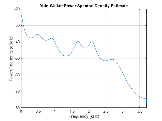
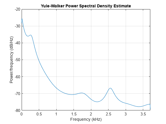
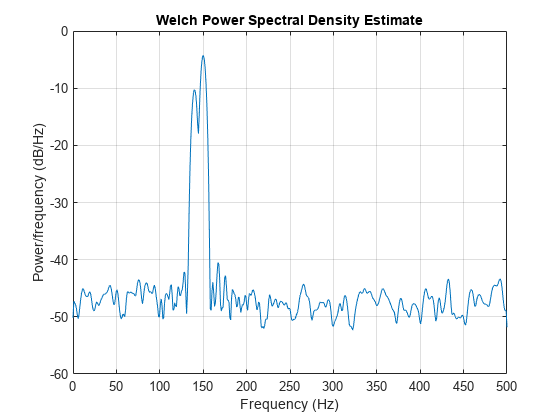
The toolbox function pyulear implements the Yule-Walker AR method. For example, compare the spectrum of a speech signal using Welch's method and the Yule-Walker AR method. Initially compute and plot the Welch periodogram.

load mtlb
pwelch(mtlb,hamming(256),128,1024,Fs)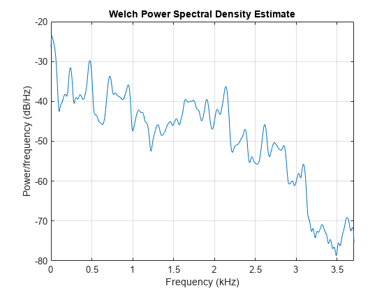

The Yule-Walker AR spectrum is smoother than the periodogram because of the simple underlying all-pole model.

order = 14;
pyulear(mtlb,order,1024,Fs)

Burg Method

The Burg method for AR spectral estimation is based on minimizing the forward and backward prediction errors while satisfying the Levinson-Durbin recursion. In contrast to other AR estimation methods, the Burg method avoids calculating the autocorrelation function, and instead estimates the reflection coefficients directly.

The primary advantages of the Burg method are resolving closely spaced sinusoids in signals with low noise levels, and estimating short data records, in which case the AR power spectral density estimates are very close to the true values. In addition, the Burg method ensures a stable AR model and is computationally efficient.

The accuracy of the Burg method is lower for high-order models, long data records, and high signal-to-noise ratios (which can cause line splitting, or the generation of extraneous peaks in the spectrum estimate). The spectral density estimate computed by the Burg method is also susceptible to frequency shifts (relative to the true frequency) resulting from the initial phase of noisy sinusoidal signals. This effect is magnified when analyzing short data sequences.

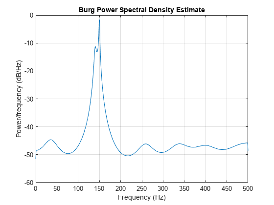
The toolbox function pburg implements the Burg method. Compare the spectrum estimates of a speech signal generated by both the Burg method and the Yule-Walker AR method. Initially compute and plot the Burg estimate.

load mtlb
order = 14;
pburg(mtlb(1:512),order,1024,Fs)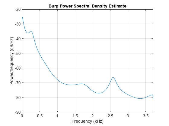

The Yule-Walker estimate is very similar if the signal is long enough.

pyulear(mtlb(1:512),order,1024,Fs)

Compare the spectrum of a noisy signal computed using the Burg method and the Welch method. Create a two-component sinusoidal signal with frequencies 140 Hz and 150 Hz embedded in white Gaussian noise of variance 0.1². The second component has twice the amplitude of the first component. The signal is sampled at 1 kHz for 1 second. Initially compute and plot the Welch spectrum estimate.

fs = 1000;
t = (0:fs)/fs;
A = [1 2];
f = [140;150];
xn = A*cos(2*pi*f*t) + 0.1*randn(size(t));

pwelch(xn,hamming(256),128,1024,fs)

Compute and plot the Burg estimate using a model of order 14.

pburg(xn,14,1024,fs)

Covariance and Modified Covariance Methods

The covariance method for AR spectral estimation is based on minimizing the forward prediction error. The modified covariance method is based on minimizing the forward and backward prediction errors. The toolbox functions pcov and pmcov implement the respective methods.

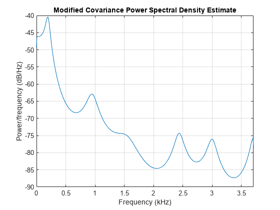
Compare the spectrum of a speech signal generated by both the covariance method and the modified covariance method. First compute and plot the covariance method estimate.

load mtlb
pcov(mtlb(1:64),14,1024,Fs)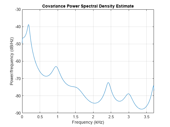

The modified covariance method estimate is nearly identical, even for a short signal length.

pmcov(mtlb(1:64),14,1024,Fs)