Nonlinearities and Noise in Idealized Baseband Mixer Block
Use the Idealized Baseband Mixer block to simulate nonlinearities and noise in your RF system design. The block uses a cubic polynomial model to simulate nonlinearities. You can plot power characteristics, Pout (dBm) vs. Pin (dBm) using Plot power characteristics button. For more information, see Plot Power Characteristics.
The Mixer block supports both phase and system noise. Frequency dependent LO phase noise vs. frequency offset is modeled in this block. This block allows you to plot phase noise magnitude response (dBc/Hz vs. Frequency) using Plot phase characteristics button. For more information, see Phase Noise in Mixer Block and Plot Phase Noise Characteristics.
Noise temperature (K), Noise figure (dB), and Noise factor parameters allows you to set the amount of system noise added to the input signal. For more information, see Mixer (System) Noise Simulations.
Nonlinearities in Idealized Baseband Mixer Block
The Mixer block uses third-order cubic polynomials to simulate nonlinearities. The model uses a linear power gain to determine the linear coefficient of a third-order polynomial and IP3, P1dB, or Psat to determine the third-order coefficient of the polynomial. The general form of cubic nonlinearity models the AM/AM characteristics as
FAM/AM(|u|) is the
magnitude of the output signal, |u| is the magnitude of the input signal,
c1 is the coefficient of the linear gain term,
and c3 is the coefficient of the cubic gain term.
The equations for IIP3, OIP3, IP1dB, OP1dB, IPsat, and OPsat are taken from [1]. The
c3 coefficient is determined as
follows.
| Type of Nonlinearity | Equations |
|---|---|
| Input third-order intercept point, IIP3 (dBm) | IIP3 is given in dBm. |
| Output third-order intercept point, OIP3 (dBm) | OIP3 is given in dBm. |
| Input 1 dB gain compression power, IP1dB (dBm) | IP1dB is given in dBm. |
| Output 1 dB gain compression power, OP1dB (dBm) | OP1dB is given in dBm and LGdB is the linear gain in dB. |
| Input saturation power, IPsat (dBm) | IPsat is given in dBm. |
| Output saturation power, OPsat (dBm) | OPsat is given in dBm. |
Plot Power Characteristics
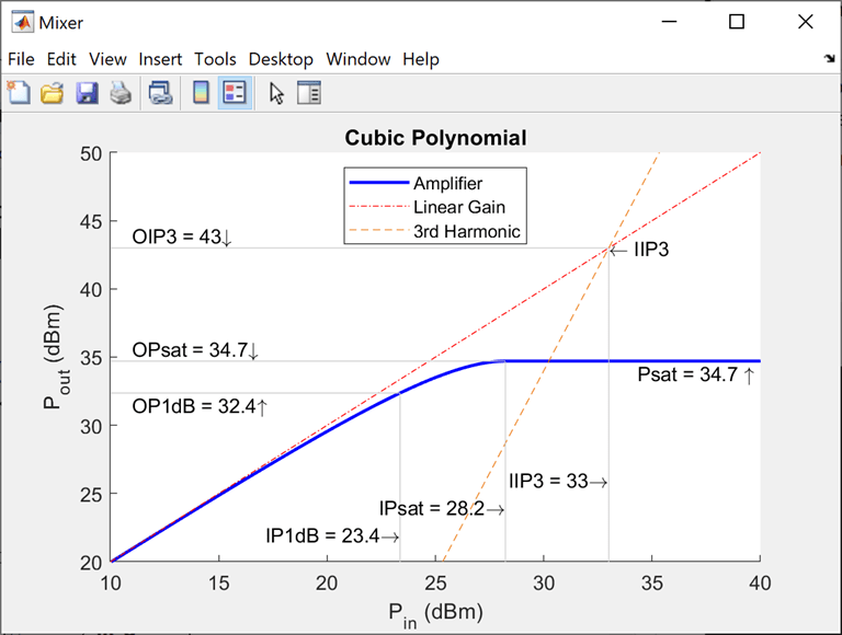
Visualize the power characteristics of your system design by using the Mixer block to
plot the Pout vs. Pin curves. For example, plot the power characteristics for a system
with a conversion gain of 10 dB and IIP3 nonlinearity. On the Main
tab, set Gain (dB) to 10. On the
Impairments tab, set Non-linearity to IIP3 and
set IIP3 (dBm) to 33. Click Plot power
characteristics on the Impairments tab.
While plotting the power characteristics in this example, set all other parameters on the Impairments tab to default values.
Phase Noise in Mixer Block
Frequency dependent LO phase noise vs. frequency offset is modeled in this block using
the MATLAB® digital filter function where the white noise input is
generated from the MATLAB random number generator randn with the
specified generator twister. The numerator and
denominator filter coefficients are derived using two methods to model
the phase noise. You can set the LO phase noise and frequency offset using the Phase noise level (dBc/Hz) and Frequency offset (Hz) parameters,
respectively.
Method one is employed for a scalar Phase noise level
(dBc/Hz) parameter and has an initial -10 dBm change in
phase noise level per frequency decade for frequencies greater than the specified Frequency offset (Hz)
[2]. Using this method, an IIR
digital filter is constructed. This is because the rational transfer function is defined
with a constant numerator coefficient and N denominator coefficients.
The number of denominator coefficients, N, is proportional to the
block sample rate / Frequency offset.
Method two is employed for vector Phase noise level
(dBc/Hz) parameter values. For modeling purposes, when the frequency is less
than the smallest specified Frequency offset (Hz) parameter
value, extrapolated phase noise values have a 1/f3
dependence. If the frequency is greater than the largest Frequency offset (Hz) parameter value, the extrapolated phase noise values
are set equal to the final Phase noise level (dBc/Hz)
vector value. Using this method, an FIR digital filter is constructed. FIR digital filter
is constructed because the rational transfer function is defined with a constant denominator
coefficient and N numerator coefficients. The number of numerator
coefficients, N, is proportional to block sample
rate / Frequency offset. To reduce spectral
leakage when simulating, an additional step is performed using an Hanning filter while
deriving the filter coefficients.
When the LO phase noise parameter, Automatic frequency resolution, is enabled, the block sample rate and frequency resolution are derived from the Frequency offset (Hz) parameter and they are used to determine the required number of filter coefficients. The number of filter coefficients can be determined using the equation
The frequency resolution is chosen to ensure that a minimum of two modeling points exist
between any two specified phase noise level points in the design. This choice for modeling
points often leads to many filter coefficients with an adverse effect on the simulation
speed. The model automatically limits the number of filter coefficients in the range
[2^5,2^16].
To improve the simulation speed, either increase the minimum distance between the Frequency offset (Hz) parameter values or disable Automatic frequency resolution and specify the Number of signal samples.
Plot Phase Noise Characteristics
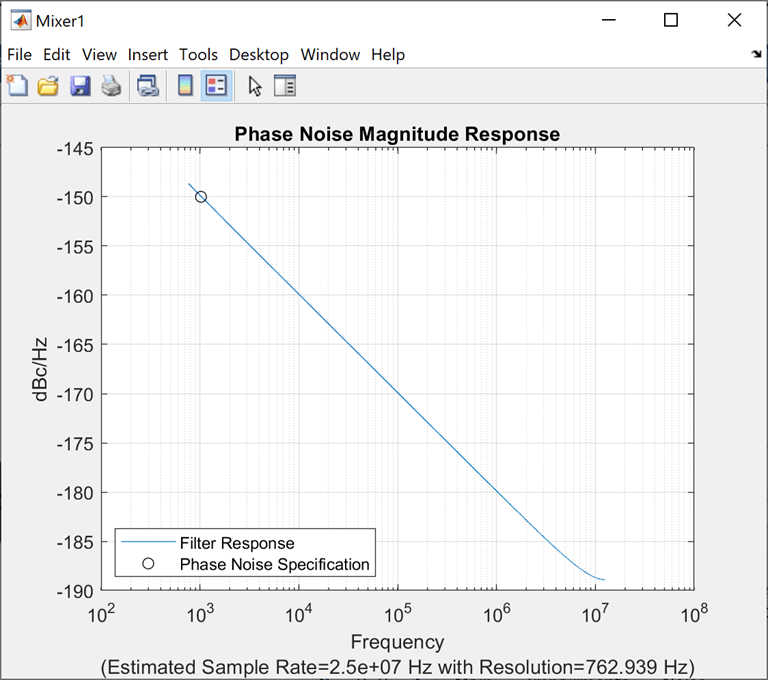
Plot the phase noise magnitude response by clicking the Plot phase characteristics button. The plot displays the phase noise specification, the design specification, and the filter response of the last simulation.
If a simulation has not been performed, the sample rate is estimated from the
Frequency offset (Hz) parameter. For the plot shown in
the table, the number of frequency bins is 4096. The number of bins can
be calculated using this equation
For example, plot the phase noise characteristics of a Mixer block. On the Noise Tab tab, set the following parameters and click Plot phase characteristics button.
Include phase noise:
OnPhase noise level (dBc/Hz):
-150Frequency offset (Hz):
1024Automatic frequency resolution:
OnSeed source:
Auto
While plotting the power characteristics in this example, set all other parameters on the Impairments tab to default values.
Mixer (System) Noise Simulations
Specify the amount of system noise added to the input signal by setting the Mixer noise type. Set one of the following:
noise-temperature— Specify the noise in kelvin. The noise added to the system is proportional to the square root ofnoise-temperature. Thenoise-temperatureis calculated using this equationnoise-factor— Specify the noise by using the equation:NF— Specify the noise in decibels relative to a noise temperature of 290 kelvin. In terms of noise factor,
References
[1] Kundert, Ken. Accurate and Rapid Measurement of IP2 and IP3. The Designer Guide Community, May 22, 2002.
[2] Kasdin, N.J. Discrete Simulation of Colored Noise and Stochastic Processes and 1/f/Sup α/ Power Law Noise Generation. Proceedings of the IEEE 83, no. 5 (May 1995): 802–27. https://doi.org/10.1109/5.381848.