Configuring an EV Simulation for Multirate HIL
This example shows an electric vehicle model suitable for multirate Hardware-In-the-Loop (HIL) deployment. The example uses the Simscape™ Network Couplers Library to split the model into separate Simulink® subsystems that can be deployed at different sample rates. This allows you to run parts of the system (for example thermal components) with a slower sample time thereby reducing overall computational cost.
Step 1: Design Model
The top-level design model is shown below. The Vehicle Control and the Driver and Environment blocks are discrete-time Simulink® subsystems running at 100Hz. The remainder of the model can be run either fixed or variable step by changing the Solver Configuration block settings.
In the design model, three thermal masses have deliberately been implemented at the top-level so that their associated time constants can be used to separate out the thermal network without changing simulation behavior.
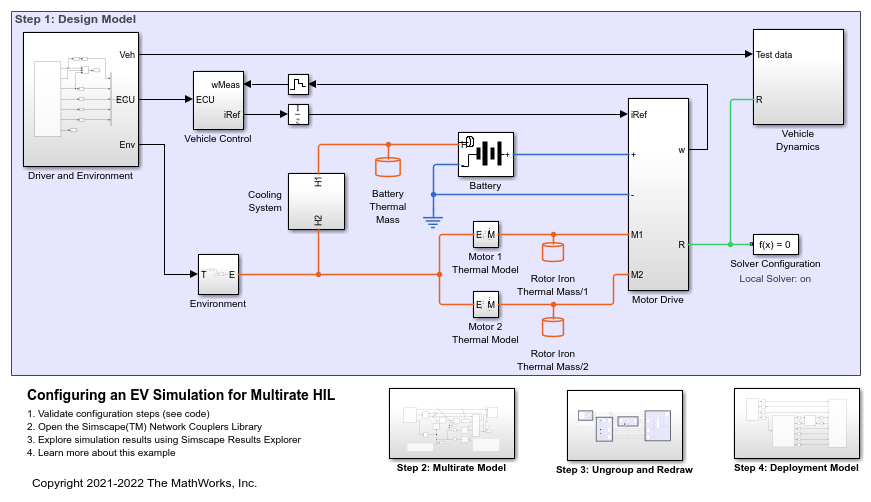
The subsystems labeled Step 1, Step 2, and Step 3 show successive steps to map from this top-level model to an implementation suitable for deployment to multirate HIL.
Step 2: Multirate Model
In this step the Simscape Network Coupler Library blocks are used to interactively experiment with good places to divide the model. From the diagram below it can be seen that the three thermal masses have been replaced with the Simscape Network Coupler Library thermal mass block. These new thermal mass blocks break the Simscape network thermal connection, replacing it with a behaviorally equivalent Simulink connection. The thermal part of the model is now a separate Simscape network, and hence another solver block is added. Because the thermal time constants are longer, the solver block is configured such that the thermal network runs five times slower than other parts of the model.
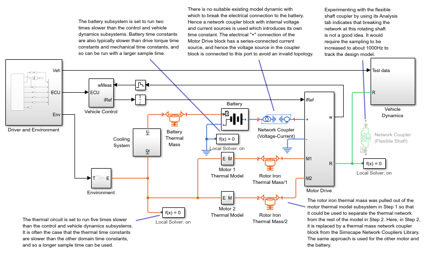
A Network Coupler (Voltage-Current) block is used to enable simulation of the battery as a separate Simscape network. The battery also does not need to be sampled at the highest rate, here being sampled at half the fastest rate. Because there is no suitable dynamic with which to break the battery connection to the Motor Drive subsystem, a numerical time constant is introduced by the Network Coupler (Voltage-Current) block. This time constant is automatically calculated based on the port sample times you specify for the block. Sample times can be iterated on until a suitable compromise between accuracy and simulation overhead is achieved.
The commented-out Network Coupler (Flexible Shaft) shows that some experimentation was done with separating out the vehicle dynamics from the motor drive dynamics. This coupler block breaks the networks with a rotational compliance, and automatically calculates a suitable stiffness based on the inertias and sample times of the two connected networks. With this it is easy to discover that sampling at about 1000Hz at the motor drive connection would be needed for reasonable accuracy, ruling this out as a place to split the model.
Step 3: Ungroup and Redraw
In this step all of the Simscape Network Coupler Library blocks are first unmasked and then their contents moved up a level using the Subsystem & Model Reference -> Expand Subsystem option from the right-click context menu. This makes the Simulink connections visible at the top level, along with the rate transition blocks. The blocks and subsystems can then be grouped together by sampling time. Here Simulink areas have been used to improve readability of the model.

Step 4: Deployment Model
In this final step each group of blocks and subsystems with a common sampling time is moved into its own subsystem. Sample time allocations can be checked by turning on sample time colors. The model is now ready for deployment to a multirate HIL platform, just in the same way as for any other Simulink model.

Simulation Results from Simscape Logging
The test run shows the vehicle accelerating to a steady speed up an incline followed by a period of descent during which electrical power is returned to the battery. It is used to show that the mapping from design model to deployment model does not introduce any significant loss of accuracy.

See Also
Network Coupler (Thermal Mass) | Network Coupler (Voltage-Current) | Network Coupler (Flexible Shaft)