Determine System Stiffness

Determining the numerical stiffness of your model helps you to decide between using an implicit or an explicit fixed-step solver for real-time simulation. To determine numerical stiffness, first use the real-time model preparation workflow to optimize the speed and accuracy of your model. Then, simulate your model using both explicit and implicit fixed-step solvers. Compare the simulation results to see how the solvers behave. If your model is numerically stiff, an explicit solver typically exhibits small oscillations around the desired solution.

Implicit solvers are more robust than explicit solvers, however, explicit solvers are faster. For robust results when performing real-time simulation with numerically stiff model, use an implicit fixed-step solver. If your model is not stiff, use an explicit solver to maximize simulation speed.

In this example, you obtain reference results by simulating a pneumatic model with a variable-step solver. You also configure and simulate the model using an implicit and then an explicit fixed-step global Simulink^® solver. Then you compare the results from all three simulations to determine if the pneumatic model is numerically stiff.

Obtain Reference Results

To open the model, at the MATLAB^® command prompt, enter:
```
ssc_pneumatic_rts_reference
```
Save the model as stiffness_model to a writable folder on the MATLAB path.
Simulate the model.
Assign the simulation results to new variables.
```
yRef = yout;
tRef = tout;
```

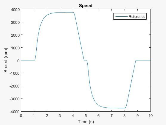
Plot the results of the variable-step simulation.

h1 = figure;
plot(tRef,yRef)
h1Leg = legend({'Reference'});
title('Speed')
xlabel('Time (s)')
ylabel('Speed (rpm)')

Simulate with an Implicit Fixed-Step Solver

Configure the model for fixed-step simulation with implicit solver ode14x. In the configuration parameters Solver pane, set:
- Type to Fixed-step
- Solver to ode14x (extrapolation)
- Under Additional options, Fixed-step size (fundamental sample time) to 1e-3
- Number of Newton's iterations to 1.
Click Apply.
Simulate the model.
Assign the simulation results to new variables.
```
yOde14x = yout;
tOde14x = tout;
```
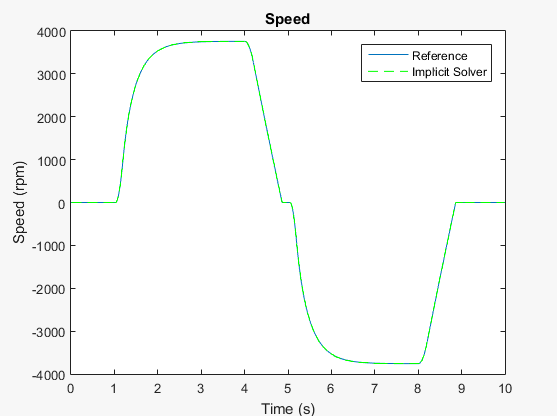
Use the stairs function to plot the results of the implicit fixed-step simulation so you can see how the solver behaves when it executes each step in the simulation.
```
h1
hold on
stairs(tOde14x,yOde14x,'g--')
h1Leg = legend({'Reference','Implicit Solver'});
```
The results appear the same.

Simulate with an Explicit Fixed-Step Solver

Configure the model for fixed-step simulation with explicit fixed-step solver ode5. In the configuration parameters Solver pane, set:
- Type to Fixed-step
- Solver to ode5 (Dormand-Prince)
Click OK.
Filter the input signal to provide the required input derivative for the explicit solver. In the Simulink-PS Converter block dialog box, set Filtering and derivatives to Filter input, derivatives calculated. Click OK.
Simulate the model.
Assign the simulation results to new variables.
```
yOde5 = yout;
tOde5 = tout;
```
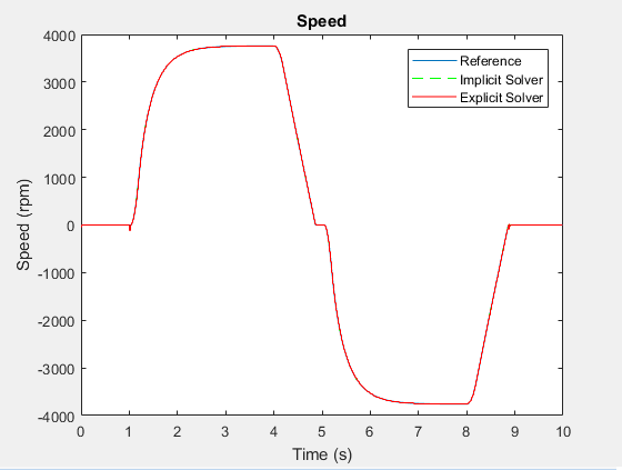
Use the stairs function to plot the results of the explicit fixed-step simulation.
```
h1
hold on
stairs(tOde5,yOde5,'r-')
h1Leg = legend({'Reference','Implicit Solver','Explicit Solver'});
```
The results differ at the inflection points.

Analyze the Results

To see the results more closely, zoom to the inflection point just after time t = ~ 1 second.

The implicit solver follows a path that is similar to the path that the variable-step solver takes when generating the reference results. The oscillations that the explicit solver exhibits indicate that the model is numerically stiff. The oscillations also indicate that the explicit solver is more computationally costly than the implicit solver for simulating the stiff model. Use a global or local implicit fixed-step solver for real-time simulation with numerically stiff models to avoid unnecessary computational cost.