Increase Simulation Speed Using the Partitioning Solver
The Partitioning solver is a Simscape™ fixed-step local solver that improves performance for certain models by reducing computational cost of simulation. Decreased computational cost yields faster simulation rates for desktop simulation and decreased task execution time (TET) for deployment. The solver converts the entire system of equations for the attached Simscape network into several smaller sets of switched linear equations that are connected through nonlinear functions. Computational cost is reduced because it is more efficient to calculate solutions for several smaller equation systems than it is to calculate the solution for one large system of equations.
The Partitioning solver does not partition models, that is it does not split a model into separate subsystems for multicore processing. To about partitioning a Simscape model, see Partition a Model By Using a Network Coupler Block.
To use the Partitioning solver, open the Solver Configuration block settings and:
Select the Use local solver check box.
Set the Solver type parameter to
Partitioning.Clear the Start simulation from steady state check box.
Set the Equation formulation parameter to
Time.
For real-time simulation, also select the Use fixed-cost runtime consistency iterations check box. For more information, see Real-Time Model Preparation.
Limitations
Not all networks can simulate with the Partitioning solver. A simulation that uses the Partitioning solver results in an error if the Simscape network cannot be represented by switched linear equations connected through nonlinear functions. Simulating with the Partitioning solver also yields an error for networks that contain:
A custom component that uses the Simscape language
delayoperator.A block that uses a discrete sample time for periodic events. Examples include the PS Counter, PS Random Number, PS Repeating Sequence, or PS Uniform Random Number blocks from the Simscape/ Physical Signals / Sources library.
Certain Solver Configuration block settings are not compatible with the Partitioning solver. A simulation that uses a Partitioning solver results in an error if the model contains a Solver Configuration block with:
Start simulation from steady state selected
Equation formulation set to
Frequency and time
Options
To further improve simulation performance, you can set the Partition
storage method parameter to Exhaustive and
specify a value for the Partition memory budget [kB] parameter,
based on the Total memory estimate data in the Statistics
Viewer. For more information, see Solver Configuration and
Partitioning Solver Statistics.
Simulate a Simscape Model Using the Partitioning Solver
% This example shows how to compare the speed and the accuracy of a
% simulation that uses the Partitioning solver to baseline results. It
% also shows how to compare the speeds of the Partitioning solver and
% the Backward Euler solver.
To open the Permanent Magnet DC Motor example and save it as a workspace variable, enter:
open_system("PermanentMagnetDCMotor")
model = 'PermanentMagnetDCMotor';

To return all simulation outputs within a single Simulink.SimulationOutput object so that you can later compare simulation times, enable the single-output format of the sim command.
% Enable single-output format
set_param(model,'ReturnWorkspaceOutputs', 'on')
Enable the signal that goes to the Motor RPM scope block for Simulink® data logging and viewing with the Simulink® Data Inspector.
% Define the w sensor subsystem and the path
%    to it as variables
rpmSensor = 'Sensing';
rpmSensorPath = [model,'/',rpmSensor];

% Mark the output signal from the w sensor subsystem
%   for Simulink(R) data logging
phRpmSensor = get_param(rpmSensorPath,'PortHandles');
set_param(phRpmSensor.Outport(1),'DataLogging','on')
The logging badge marks the signal in the model.

Run timed simulations for each of these solvers:
Variable-step global solver, the original solver for the model
Fixed-step local Backward Euler solver
Fixed-step local Partitioning solver
% Define the Solver Configuration block and the path
%    to it as variables
solvConfig = 'Solver Configuration';
solvConfigPath = [model,'/',solvConfig];

% Run a timed simulation using the original solver
out = sim(model);
tBaseline = out.SimulationMetadata.TimingInfo.ExecutionElapsedWallTime;

% Select option Solver Configuration >  Use local solver
set_param(solvConfigPath, 'UseLocalSolver', 'on')

% Set Solver Configuration >  Solver type > Partitioning
set_param(solvConfigPath, 'LocalSolverChoice',...
    'NE_PARTITIONING_ADVANCER')

% Run a timed simulation using the Partitioning solver
out = sim(model);
tPartition = out.SimulationMetadata.TimingInfo.ExecutionElapsedWallTime;

% Set Solver Configuration >  Solver type > Backward Euler
set_param(solvConfigPath, 'UseLocalSolver', 'on',...
    'LocalSolverChoice','NE_BACKWARD_EULER_ADVANCER')

% Run a timed simulation using the Backward Euler solver
out = sim(model);
tBackEuler = out.SimulationMetadata.TimingInfo.ExecutionElapsedWallTime;

% Compute the percent difference for the simulation times
spdPartitionVsBaseline = 100*(tBaseline - tPartition)/tBaseline;
spdBackEulerVsBaseline = 100*(tBaseline - tBackEuler)/tBaseline;
spdPartitionVsBackEuler = 100*(tBackEuler - tPartition)/tBackEuler;

% Reset the solver to the original setting by deselecting Use local solver
set_param(solvConfigPath, 'UseLocalSolver', 'off')
compTimeDiffTable = table({'Baseline';...
    'Partitioning';...
    'Backward Euler'},...
    {tBaseline;tPartition;tBackEuler},...
'VariableNames', {'Solver','Sim_Duration'});

display(compTimeDiffTable);
compTimeDiffTable =

  3×2 table

          Solver          Sim_Duration
    __________________    ____________

    {'Baseline'      }     {[0.1098]}
    {'Partitioning'  }     {[0.0114]}
    {'Backward Euler'}     {[0.0189]}
compPctDiffTable = table({'Partitioning versus Baseline';...
    'Backward Euler versus Baseline';...
    'Partitioning versus Backward Euler'},...
    {spdPartitionVsBaseline;...
    spdBackEulerVsBaseline;...
    spdPartitionVsBackEuler},...
'VariableNames', {'Comparison','Percent_Difference'});

display(compPctDiffTable);
compPctDiffTable =

  3×2 table

                  Comparison                  Percent_Difference
    ______________________________________    __________________

    {'Partitioning versus Baseline'      }       {[89.5812]}
    {'Backward Euler versus Baseline'    }       {[82.7700]}
    {'Partitioning versus Backward Euler'}       {[39.5307]}
Simulation time on your machine may differ because simulation speed depends on machine processing power and the computational cost of concurrent processes.
The local fixed-step Partitioning and Backward Euler solvers are faster than the variable-step baseline solver. The Partitioning solver is typically, but not always, faster than the Backward Euler solver.
To compare the results, open the Simulink® Data Inspector.
% Get Simulink Data Inspector run IDs for
%    the last three runs
runIDs = Simulink.sdi.getAllRunIDs;
runBaseline = runIDs(end - 2);
runPartition = runIDs(end - 1);
runBackEuler = runIDs(end);

% Open the Simulink Data Inspector
Simulink.sdi.view

compBaselinePartition = Simulink.sdi.compareRuns(runBaseline,...
    runPartition);
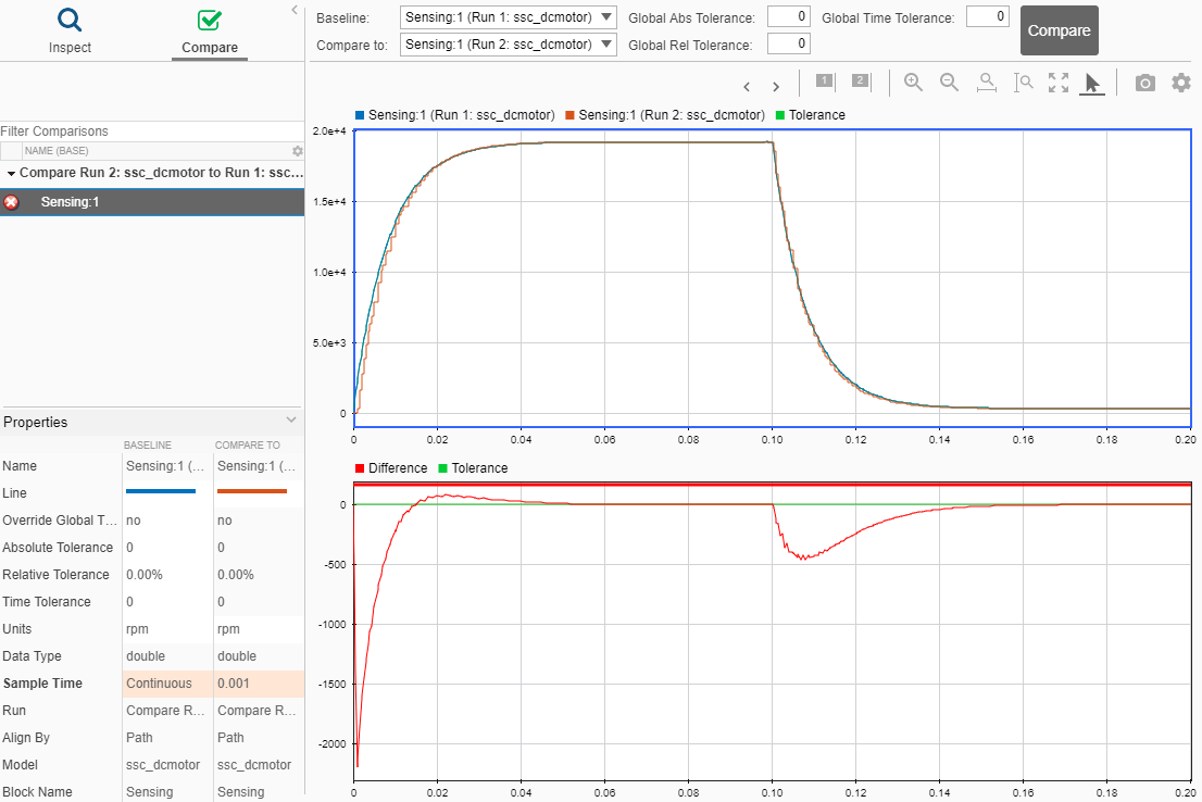
To see the comparison, click Compare and then click Sensing 1.

The first plot shows the overlay of the baseline and Partitioning solver simulation results. The second plot shows how they differ. The default tolerance for differences is 0. To determine if the accuracy of the results meet your requirements, you can adjust the relative, absolute, and time tolerances.