Solver Configuration

R2026b

Physical network environment and solver configuration

• 

Solver Configuration block

To add a block to a model, double-click the canvas and start typing the block name. Then, select the block from the list.

Libraries:
Simscape / Utilities

Description

The Solver Configuration block defines the solver and numerical settings required to simulate the connected Simscape physical network. Each physical network represented by a connected Simscape™ block diagram requires one Solver Configuration block. The Solver Configuration block specifies the solver parameters that your model needs to begin simulation.

Examples

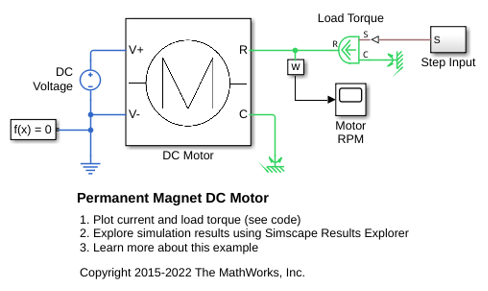
Permanent Magnet DC Motor

Verify manufacturer specifications of no-load speed, no-load current, and stall torque for a DC motor by using a test harness and Simscape™ blocks.

• Open Model

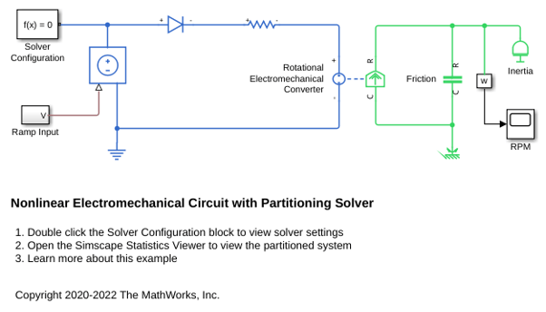
Nonlinear Electromechanical Circuit with Partitioning Solver

Models a DC Motor controlled by a ramp input. The resulting system of equations contains switched linear and nonlinear elements brought about by the Diode and Rotational Friction blocks respectively. However, the Partitioning solver is able to convert this system into several smaller sets of linear time-invariant and switched linear equations connected by nonlinear functions. This helps in reducing computational cost, which in turn yields faster simulation.

• Open Model

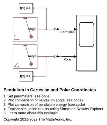
Pendulum in Cartesian and Polar Coordinates

Two different implementations of a planar pendulum.

• Open Model

Ports

Conserving

Port_1 — Connection port

untyped conserving port

Untyped conserving port associated with the connection port. Connect this port to a connection line between conserving ports of any type.

Parameters

Equation formulation — Equation formulation option

Time (default) | Frequency and time

Option to formulate equations in the time domain or in combined frequency–time domains.

Use the Frequency and time value to speed up simulation for systems that have a single nominal frequency. For more information, see Frequency and Time Simulation Mode.

Index reduction method — Index reduction method

Derivative replacement (default) | Projection | None

Index reduction method to use for nonlinear, high-index differential algebraic equations (DAEs). Select from these options:

• Derivative replacement — The solver differentiates parts of the DAE analytically and appends them to the original system. For each additional equation, the solver replaces a derivative with a new algebraic variable called a dummy derivative. For more information, see https://epubs.siam.org/doi/abs/10.1137/0914043?journalCode=sjoce3.

• Projection — Use this option if the Derivative replacement method fails due to issues with dynamic state selection.

• None — If your model does not contain nonlinear high-index DAEs, use this option to bypass nonlinear index reduction and remove the analysis overhead.

Start simulation from steady state — Steady state option

off (default) | on

Option to start the simulation from steady state. When you clear this parameter, simulation starts from the initial state obtained from the initial conditions computation.

When you select this parameter, the solver attempts to find the steady state that results if the inputs to the system are constant for a sufficiently large time. For more information, see Initial Conditions Computation. Simulation then starts from this steady state.

For models compatible with frequency-and-time equation formulation, when you select this check box, the solver attempts to perform sinusoidal steady-state initialization. The solver performs initialization by using frequency-time equations, and the simulation uses the equation formulation and other options selected in the Solver Configuration block. For more information, see Frequency and Time Simulation Mode.

Note

Selecting the Initial state parameter on the Data Import/Export pane of the Configuration Parameters dialog box overrides the Start simulation from steady state option.

Consistency tolerance — State-based tolerance method

Model AbsTol and RelTol (default) | Local tolerance settings

State-based tolerance method to determine initial conditions and compute the transient initialization. Select from these options:

• Model AbsTol and RelTol — Use the model tolerance settings specified by the Absolute tolerance and Relative tolerance parameters in the Solver pane of the Configuration Parameters dialog box.

• Local tolerance settings — Replace the model tolerance settings with local values.

Absolute tolerance — Local absolute tolerance

0.001 (default) | positive scalar

Local absolute tolerance that the solver uses to compute the initial conditions and transient initialization conditions.

Dependencies

To enable this parameter, set Consistency tolerance to Local tolerance settings.

Relative tolerance — Local relative tolerance

0.001 (default) | positive scalar

Local relative tolerance that the solver uses to compute the initial conditions and transient initialization conditions.

Dependencies

To enable this parameter, set Consistency tolerance to Local tolerance settings.

Tolerance factor — Scaling factor for absolute and relative tolerances

0.001 (default) | scalar in the range (0,1]

Scaling factor for the state-based absolute and relative tolerances. Scaling factor for the state-based absolute and relative tolerances. The block applies this value on top of the settings you specify for the model or local tolerances. Decreasing this value improves accuracy, but can reduce simulation performance or cause the simulation to fail if the value is too small. Increasing this value can improve performance at the expense of accuracy.

Use local solver — Sample-based local solver option

off (default) | on

Option to use a sample-based local solver. In sample-based simulation, Simulink^® treats all of the continuous physical network states as discrete states. The solver updates the states once per time step. Use this option for real-time and hardware-in-the-loop simulation. When you select this parameter, the local solver settings apply only to the Simscape physical network connected to this block. The rest of the model uses the Simulink solver.

Note

When you enable this parameter, minimizing the use of Simulink or Simulink Control Design™ linearization tools may improve performance.

Solver type — Solver to use for local simulation

Backward Euler (default) | Trapezoidal Rule | Partitioning

Solver type to use for local simulation. Select from these options:

• Backward Euler — This solver damps out oscillations, but is more stable, especially if you increase the time step.

• Trapezoidal Rule — This solver captures oscillations better than the Backward Euler setting, but is less stable.

• Partitioning — This solver increases real-time simulation speed by partitioning the system of equations that correspond to a Simscape network into a cascade of smaller equation systems. This solver provides a significant increase in real-time simulation speed. For more information, see Understanding How the Partitioning Solver Works and Increase Simulation Speed Using the Partitioning Solver.

Regardless of which setting you choose, the solver uses the Backward Euler method:

• At the start of simulation.

• After an instantaneous change, such as when a block undergoes an internal discrete change. These changes include clutches locking and unlocking, valve actuators opening and closing, or the switching of the PS Asynchronous Sample & Hold block.

Dependencies

To enable this parameter, select Use local solver.

Sample time — Sample time for the local solver

0.001 (default) | positive scalar

Local solver sample time, in seconds. The solver updates the states once per time step. Balance the value of this parameter with the value of the Nonlinear iterations parameter. To learn more, see Define Step Size and Number of Nonlinear Iterations for Simscape Real-Time Simulation.

Dependencies

To enable this parameter, select Use local solver.

Partition method — Partition method

Balanced simulation (balance nonlinearities and stability) (default) | Stable simulation (maximize stability) | Fast simulation (minimize nonlinearities)

Option to prioritize speed or robustness when using the Partitioning local solver:

• Stable simulation (maximize stability) — Improve simulation robustness by maximizing the use of implicit solvers for groups of equations.

• Balanced simulation (balance nonlinearities and stability) — Balance speed and robustness by increasing the use of implicit solvers for groups of equations.

• Fast simulation (minimize nonlinearities) — Improve simulation performance by maximizing the use of explicit solvers for groups of equations.

Dependencies

To enable this parameter, select Use local solver and set Solver type to Partitioning.

Partition storage method — Partition storage method

As needed (default) | Exhaustive

Method to use to store the partition data. When you use the Partitioning solver, it solves the small switched linear equations consecutively. You can choose to store the matrix inverses or to improve the simulation performance. Then, if the solver detects the same configuration in a subsequent time step, the partitioning solver uses the stored matrix inverses, instead of recomputing them. Select from these options:

• As needed — Compute matrix inverses during simulation. This method does not require as much memory but can result in performance variability.

• Exhaustive — Compute and store matrix inverses before simulation. This method improves the simulation performance but requires more memory. Use the Partition memory budget [kB] parameter to specify the maximum allowed memory budget for the data.

Dependencies

To enable this parameter, select Use local solver and set Solver type to Partitioning.

Partition memory budget [kB] — Memory budget for exhaustive partitioning storage

1024 (default) | positive scalar

Memory budget for exhaustive partitioning, in kB. The solver generates an error when it exceeds the budget. Adjust the value based on your available memory resources and on the Total memory estimate data in the Statistics Viewer. For more information, see Partitioning Solver Statistics.

Dependencies

To enable this parameter

• Select the Use local solver parameter.

• Set Solver type to Partitioning.

• Set Partition storage method to Exhaustive.

Resolve indeterminate equations during runtime — Option to use runtime regularization to solve indeterminate systems

on (default) | off

Option to use runtime regularization to solve statically indeterminate systems. Certain model configurations, such as parallel clutches that lock, or current sensors that connect in parallel, allow an infinite number of solutions, which makes them statically indeterminate. Select this parameter to enable regularization, which is a transformation that converts models with indeterminate Through variables into solvable systems. This parameter is enabled by default.

If your model does not contain configurations with lossless parallel flow paths, you can speed up simulation by clearing the Resolve indeterminate equations during runtime parameter.

Dependencies

To enable this parameter, select the Use local solver parameter and set Solver type to either Backward Euler or Trapezoidal.

Use fixed-cost runtime consistency iterations — Fixed-cost simulation option

off (default) | on

Option to compute the transient initialization and solver phase at a fixed cost. When you select this parameter, you can specify the number of nonlinear and mode iterations to use for the transient initialization and solver computations. If the system does not converge when it performs the specified number of iterations, the solver proceeds to the next step.

When you clear this setting, the solver performs as many iterations as necessary to reach convergence and generates an error if it fails to reach convergence at the time of transient initialization. When you use this setting, the solver always computes impulses.

For more information, see Making Optimal Solver Choices for Physical Simulation.

Nonlinear iterations — Number of Newton iterations for transient initialization

3 (default) | positive integer

Number of Newton iterations that the solver uses during the transient initialization and integration steps. The solver completes the specified number of Newton iterations regardless of convergence. You can use the simscape.getLocalSolverFixedCostInfo function to find the necessary iterations per step. Balance the value of this parameter with the value of the Sample time parameter. To learn more, see Define Step Size and Number of Nonlinear Iterations for Simscape Real-Time Simulation.

Dependencies

To enable this parameter, select Use fixed-cost runtime consistency iterations.

Mode iterations — Number of mode iterations for transient initialization

2 (default) | positive integer

Number of mode iterations to perform at the time of transient initialization.

Dependencies

To enable this parameter, select Use fixed-cost runtime consistency iterations and clear Use local solver.

Compute impulses — Option to compute impulses

off (default) | on

Option to compute impulses during transient initialization for both global and local fixed-cost solvers. Computing impulses can significantly improve simulation speed for models that have switching events, contact events, and changes in constraints. However, computing impulses raises the transient initialization cost proportionally to the number of impulse iterations. When you clear Use fixed-cost runtime consistency iterations, the solver always computes impulses.

When you select Compute impulses, you specify the number of impulse iterations to perform in Impulse iterations. If the impulse computation does not converge in the specified number of iterations, the solver proceeds to the next step.

When you clear Compute impulses, the solver does not perform impulse iterations.

Dependencies

To enable this parameter, select Use fixed-cost runtime consistency iterations.

Impulse iterations — Number of impulse iterations for transient initialization

2 (default) | positive integer

Number of impulse iterations to perform at the time of transient initialization. If the system does not converge after reaching this value, it proceeds to the next step.

Dependencies

To enable this parameter, select the Compute impulses parameter.

Maximum threads for function evaluation — Maximum number of function evaluation threads

1 (default) | positive integer

Maximum number of threads to use for multithread function evaluation during real-time simulation. You can use multithreading for the Backward Euler and Trapezoidal solvers. The actual number of threads that the block uses is the nearest power of 2 that does not exceed the parameter value. For example, set this parameter to 5, the solver uses four threads. The default value, 1, corresponds to single-thread function evaluation.

Multithread function evaluation does not support frequency-and-time simulation, delays, scalable compilation, accelerator mode, or rapid accelerator mode. You can only generate code by using Simulink Real-Time™ when using multithread function evaluation.

Dependencies

To enable this parameter

• Select Use local solver.

• Clear Resolve indeterminate equations during runtime.

• Set Solver type to Backward Euler or Trapezoidal.

• Select Use fixed-cost runtime consistency iterations.

Linear Algebra — Method to use for matrices

auto (default) | Sparse | Full

Method that the solver uses to handle matrix algebra. Select from these options:

• auto — The solver automatically selects the appropriate option, either sparse or full, for treating the matrices.

• Sparse — The solver treats matrices as sparse.

• Full — The solver treats matrices as full.

Number of threads (specify n for 2^n) — Number of threads

0 (default) | nonnegative integer

Number of threads to use for multithread linear algebra, specified as 2ⁿ, where n is the value of this parameter. The default value of 0 corresponds to single-thread linear algebra.

For small models, multithread algorithms that use values greater than 0 may be slower than single-thread.

Dependencies

To enable this parameter, select the Use local solver parameter and set the Linear algebra parameter to Sparse.

Delay memory budget [kB] — Memory budget for processing delays

1024 (default) | positive scalar

Maximum memory budget, in KB, that the block uses for processing delays. The block adheres to this budget when simulating models that contain blocks from the Delays library or custom blocks that use the delay Simscape language construct. This budged protects against excessive memory swapping. If the simulation exceeds the budget, the Solver generates an error.

Apply filtering at 1-D/3-D connections when needed — Option to apply filtering between 1-D and 3-D ports

on (default) | off

Option to apply filtering at connections between the 1-D connections of Simscape blocks and 3-D connections in other products, such as Simscape Multibody™ and other add-on products. Use the Statistics Viewer to determine whether your model has connections between 1-D and 3-D ports. For more information, see 1-D/3-D Interface Statistics.

When you connect a Simscape Multibody block directly to a Simscape network, the solver may require an additional derivative. When you select this parameter, the solver automatically applies input filtering to the signal entering the Simulink-PS Converter block to obtain this additional derivative. The Filtering time constant parameter provides the time constant for the delay.

Note

If you clear this parameter and the 1-D/3-D connection requires the additional derivative, the solver generates an error message.

Filtering time constant — Delay time constant

0.001 (default) | positive scalar

Delay filtering time constant, in seconds, for connections between 1-D and 3-D ports. The parameter value applies to all connections attached to the same Solver Configuration block.

Dependencies

To enable this parameter, select the Apply filtering at 1-D/3-D connections when needed parameter.

Multibody

Use local solver — Option to use sample-based local solver

off (default) | on

Option to use a sample-based local solver for the connected Simscape Multibody network. Using a local solver can reduce the computational cost for a complex Simulink model that has simple Simscape Multibody networks. If you select this parameter, the Simscape Multibody network appears to the global Simulink solver with discrete states. The local solver updates the states once per time step.

Note

This parameter is independent from the Use local solver parameter in the Main tab of the block dialog box, which applies to the Simscape network connected to the block.

Solver type — Multibody solver type

First-order explicit formula (default) | Second-order explicit formula | Third-order explicit formula | Fourth-order explicit formula | Fifth-order explicit formula | Eighth-order explicit formula

Solver to use to update the states in the Simscape Multibody network. Select from these options:

• First-order explicit formula — Explicit fixed-step solver that uses the same mathematical equations as ode1.

• Second-order explicit formula — Explicit fixed-step solver that uses the same mathematical equations as ode2.

• Third-order explicit formula — Explicit fixed-step solver that uses the same mathematical equations as ode3.

• Fourth-order explicit formula — Explicit fixed-step solver that uses the same mathematical equations as ode4.

• Fifth-order explicit formula — Explicit fixed-step solver that uses the same mathematical equations as ode5.

• Eighth-order explicit formula — Explicit fixed-step solver that uses the same mathematical equations as ode8.

Dependencies

To enable this parameter, in the Multibody section, select the Use local solver parameter.

Sample time — Sample time for the Multibody local solver

0.001 (default) | positive scalar

Sample time for the Multibody local solver, in seconds. The solver updates the states of the connected Simscape Multibody network once per time step.

Dependencies

To enable this parameter, in the Multibody section, select the Use local solver parameter.

Extended Capabilities

C/C++ Code Generation
Generate C and C++ code using Simulink® Coder™.

Version History

Introduced in R2007a

R2026b: Use new partitioning methods

You can set the Partitioning method parameter to one of these options:

• Stable simulation (maximize stability) — Improve simulation robustness by maximizing the use of implicit solvers for groups of equations.

• Balanced simulation (balance nonlinearities and stability) — Balance speed and robustness by increasing the use of implicit solvers for groups of equations.

• Fast simulation (minimize nonlinearities) — Improve simulation performance by maximizing the use of explicit solvers for groups of equations.

The Robust simulation option has been renamed to Balanced simulation (balance nonlinearities and stability). Simscape updates models from prior versions to use the new option.

R2026b: Use multithreading for Trapezoidal solver

To apply multithread function evaluation when using the Trapezoidal solver, set Maximum threads for function evaluation to a value greater than 1.

R2024a: Control runtime regularization independently of fixed-cost simulation

The Resolve indeterminate equations check box in the Solver Configuration blocks, which applies runtime regularization to solve statically indeterminate systems, has been renamed to Resolve indeterminate equations during runtime and moved to a different section of the dialog box. Previously, you needed to select the Use fixed-cost runtime consistency iterations check box to enable it. Now, to enable the Resolve indeterminate equations during runtime check box, you need to select the Use local solver check box and set Solver type to either Backward Euler or Trapezoidal Rule. Unless your model contains lossless parallel flow paths, such as ideal parallel clutches or switches, you can now clear the Resolve indeterminate equations during runtime check box and speed up simulation whenever you use these types of local solver, independently of whether the simulation is fixed-cost or not.

You can no longer turn off runtime regularization for global solvers.

R2023b: Multibody local solver

The new Multibody section contains settings and parameters specific to solving the connected Simscape Multibody network. The Use local solver check box lets you reduce the computational cost by representing the Simscape Multibody network as if it has discrete states. The Solver type and Sample time parameters in this section apply to the Multibody local solver only.

R2022b: New ways to specify consistency tolerance

The block uses state-based absolute and relative consistency tolerances, multiplied by a scaling factor, to compute the initial conditions and for transient initialization. The Consistency tolerance parameter lets you select between the model tolerances or the local tolerance settings. The new Tolerance factor parameter provides a scaling factor for these values. This state-based method provides better robustness and efficiency, especially if used in conjunction with scaling the model by nominal values.

In previous releases, the Consistency tolerance parameter had a numeric value, and the block used a nonlinear solver based on the equation residual tolerance to initialize the model.

If you open an existing model where the Consistency tolerance parameter has a numeric value, the model continues to use the same residual-based computation method that it used in previous releases. Your simulation results do not change.

To upgrade your existing models to use the state-based method, use the Check Simscape use of state-based consistency tolerances check in the Upgrade Advisor.

R2022b: Multithread function evaluation for fixed-cost simulation

If your model uses the Backward Euler local solver, computing Newton iterations is time-consuming and may present an issue for fixed-cost simulations. You can use multithread function evaluation to speed up simulation on a multicore machine by using the new Maximum threads for function evaluation parameter and clearing the new Resolve indeterminate equations check box.

In previous releases, the solver used single-thread function evaluation and always applied runtime regularization. The default values of the Maximum threads for function evaluation parameter and Resolve indeterminate equations check box are equivalent to the algorithm used in previous releases.