Developing the Apollo Lunar Module Digital Autopilot

R2026b

"Working on the design of the Lunar Module digital autopilot was the highlight of my career as an engineer. When Neil Armstrong stepped off the LM (Lunar Module) onto the moon's surface, every engineer who contributed to the Apollo program felt a sense of pride and accomplishment. We had succeeded in our goal. We had developed technology that never existed before, and through hard work and meticulous attention to detail, we had created a system that worked flawlessly." -Richard J. Gran, The Apollo 11 Moon Landing: Spacecraft Design Then and Now.

This example demonstrates the Lunar Module digital autopilot for attitude control during the Descent Orbit Insertion phase of the Apollo 11 mission, showing how the original design team could have done it using Simulink® and Aerospace Blockset™ if they had been available in 1961.

Model Description

Developing the autopilot in Simulink takes a fraction of the time it took for the original design of the Apollo Lunar Module autopilot.

open_system("aero_dap3dof");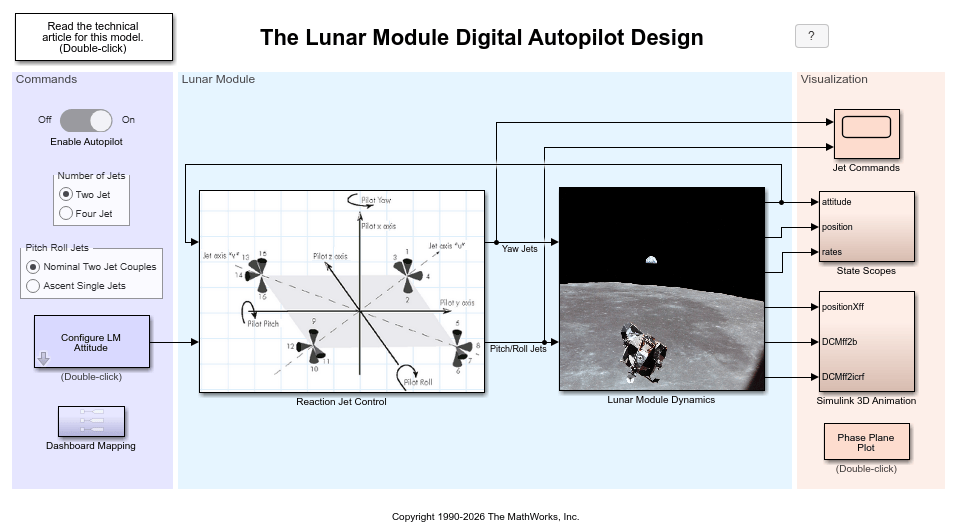

The Reaction Jet Control subsystem models the digital autopilot designed by George Cherry at MIT Instrumentation Laboratories (MIT IL), now called Draper Laboratory. The autopilot maintains commanded attitude using reaction control jets in a bang-bang control mode where jets are either fully on or fully off, with no intermediate throttle. When attitude error grows too large, the autopilot fires jets to apply corrective torque and drive the spacecraft back toward the desired orientation. Once the error is small enough, jets turn off and the spacecraft coasts freely until correction is needed again. This approach minimizes a weighted mix of response time and fuel consumption [2]. A Stateflow® diagram implements this control logic, with the Lunar Module state machine executing in either a Fire_region or a Coast_region. The diagram evaluates the current attitude error and rate to determine transitions between these regions and computes which specific jets to fire.

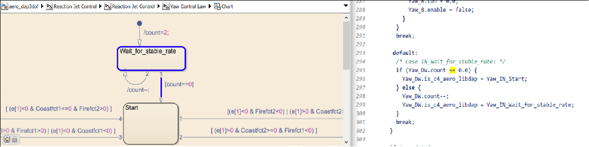
The below image shows a portion of the LM autopilot yaw control law. The control law is implemented in Stateflow, enabling engineers to work with executable finite state machines instead of writing the textual code. The source code, shown next to the state machine, is automatically generated from the model and includes traceability to the model components (highlighted in blue).

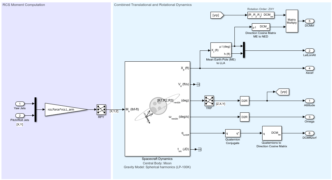
The Lunar Module Dynamics subsystem captures how the spacecraft moves and rotates in response to reaction jet firings and lunar gravity using the Spacecraft Dynamics block configured with Moon spherical harmonic gravity for orbit propagation and vehicle inertia for attitude response. The Visualization area of the model provides three ways to observe autopilot performance during simulation: a phase plane plot showing the controller state trajectory against the fire/coast switch curves, Simulink scopes displaying the commanded attitude signal alongside measured attitude and body rates over time, and a Simulink 3D Animation viewer rendering the Lunar Module in lunar orbit. Run the model to observe how the digital autopilot acquires and maintains the commanded attitude.

In the phase plane plot, parabolic switch curves (attitude error vs. rate error) divide the state space into fire and coast regions. When the state trajectory crosses a fire boundary, jets turn on to drive the error toward the deadband. When it crosses a coast boundary, jets turn off and the spacecraft drifts freely. The deadband is the ±0.345 degree region between the fire and coast switch curves where no jets fire. The coast switch curves use an effective acceleration one-tenth that of the fire switch curves, creating a separation (hysteresis) between the two boundaries. This prevents the jets from rapidly cycling on and off as the state approaches the switching threshold.

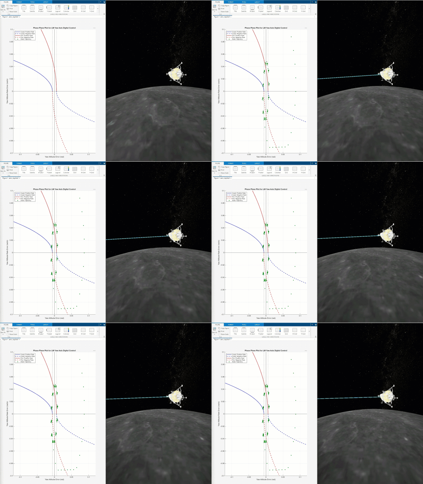
Simulink 3D Animation™ viewer shows the Lunar Module rotating above the lunar surface as the reaction control jets fire to acquire and hold the commanded attitude.

Interactive Controls

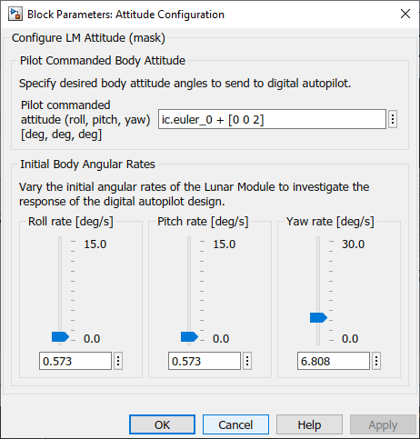
To interact with the Lunar Module model, vary autopilot settings and Lunar Module initial states in the Commands area. For example, to observe how the digital autopilot design handles increased initial body rates, use the slider components in Configure LM Attitude.

Mission Description

The LM digital autopilot has three degrees of freedom. This means that by design, the reaction jet thrusters are configured and commanded to rotate the vehicle without impacting the vehicle's orbital trajectory. Therefore, the translational dynamics in his model are approximated via orbit propagation using the Spacecraft Dynamics block from Aerospace Blockset. The block is configured to use Moon spherical harmonic gravity model LP-100K.

To demonstrate the digital autopilot design behavior, the "Descent Orbit Insertion" mission segment, just prior to the initiation of the powered descent, was selected from the Apollo 11 Mission Report.

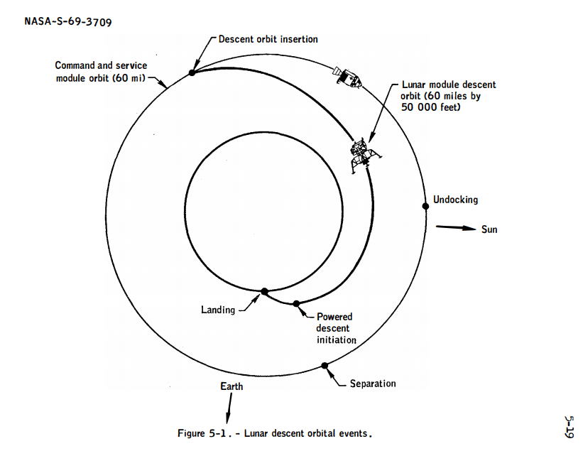
(Image Credit: NASA)

The "Descent Orbit Insertion" burn began 101 hours, 36 minutes, and 14 seconds after lift-off and lasted 30 seconds. The burn set the Lunar module on a trajectory to lower its orbit from approximately 60 nautical miles to 50,000 ft over about an hour. At 50,000 ft, the Module initiated its powered descent.

Initialize the model aero_dap3dof with the approximate trajectory of the Lunar Module immediately after the descent orbit insertion burn.

mission.t_rangeZero             = datetime(1969,7,16,13,32,0); % lift-off
mission.t_descentInsertionStart = mission.t_rangeZero + hours(101) + minutes(36) + seconds(14);
mission.t_descentInsertion      = mission.t_descentInsertionStart + seconds(30);
mission.t_poweredDescentStart   = mission.t_rangeZero + hours(102) + minutes(33) + seconds(5.2);

disp(timetable([mission.t_rangeZero, mission.t_descentInsertionStart, ...
    mission.t_descentInsertion, mission.t_poweredDescentStart]', ...
    {'Range Zero (lift-off)', 'Descent Orbit Insertion (Engine ignition)', ...
    'Descent Orbit Insertion (Engine cutoff)', 'Powered Descent (Engine ignition)'}', VariableNames="Mission Phase"));

            Time                            Mission Phase                
    ____________________    _____________________________________________

    16-Jul-1969 13:32:00    {'Range Zero (lift-off)'                    }
    20-Jul-1969 19:08:14    {'Descent Orbit Insertion (Engine ignition)'}
    20-Jul-1969 19:08:44    {'Descent Orbit Insertion (Engine cutoff)'  }
    20-Jul-1969 20:05:05    {'Powered Descent (Engine ignition)'        }

The trajectory of the module at "Descent Orbit Insertion (Engine cutoff)" and "Powered Descent Initiation (Engine ignition)" is provided in the Apollo 11 Mission Report (Table 7-II.- Trajectory Parameters).

mission.Latitude_deg  = [-1.16, 1.02]';    % [deg]
mission.Longitude_deg = [-141.88, 39.39]'; % [deg]
mission.Altitude_mi   = [57.8, 6.4]';      % [nautical miles]
mission.Altitude_ft   = convlength(mission.Altitude_mi, 'naut mi', 'ft');
mission.Velocity_fps  = [5284.9, 5564.9]'; % [ft/s] (in Inertial frame)
mission.FlightPathAngle_deg = [-0.06, 0.03]'; % [deg] (measured upward from local horizontal plane)
mission.HeadingAngle_deg = [-75.19 -101.23]'; % [deg] (measured East of North)
disp(table({'Range Zero (lift-off)'; 'Descent Orbit Insertion (Engine ignition)'}, ...
    mission.Latitude_deg, mission.Longitude_deg, mission.Altitude_mi, ...
    mission.Velocity_fps, mission.FlightPathAngle_deg, mission.HeadingAngle_deg, ...
    VariableNames=["Mission Phase", ...
    "Latitude (deg)", "Longitude (deg)", "Altitude (mi)", ...
    "Velocity (ft/s)", "Flight path angle (deg)", "Heading (deg)"]));

                    Mission Phase                    Latitude (deg)    Longitude (deg)    Altitude (mi)    Velocity (ft/s)    Flight path angle (deg)    Heading (deg)
    _____________________________________________    ______________    _______________    _____________    _______________    _______________________    _____________

    {'Range Zero (lift-off)'                    }        -1.16             -141.88            57.8             5284.9                  -0.06                 -75.19   
    {'Descent Orbit Insertion (Engine ignition)'}         1.02               39.39             6.4             5564.9                   0.03                -101.23   

Model Initialization

Initialize model parameters for the mission phase "Descent Orbit Insertion (Engine cutoff)" using the data defined above.

The initialization function aero_dap3dofdata requires information about the orientation of the Moon, which can be calculated using the Aerospace Toolbox function moonLibration. This function requires "Ephemeris Data for Aerospace Toolbox". Use aeroDataPackage to install this data if it is not already installed.

mission.LibrationAngles_deg = moonLibration(juliandate(mission.t_descentInsertion), "405");

This example uses saved libration angle data corresponding with t_descentInsertion. Use the above command after installing the required ephemeris data.

mission.LibrationAngles_deg = [0.006379917345247; 0.382328074214300; 6.535718297208969];

Run the initialization function:

[moon, ic, vehicle, rcs] = aero_dap3dofdata(...
    mission.Latitude_deg(1), mission.Longitude_deg(1), mission.Altitude_ft(1), ...
    mission.Velocity_fps(1), mission.FlightPathAngle_deg(1), ...
    mission.HeadingAngle_deg(1), mission.LibrationAngles_deg);

Closing Remarks

Building a digital autopilot was a daunting task in 1961 because there was very little industrial infrastructure for it - everything about it was in the process of being invented. Here is an excerpt from the technical article The Apollo 11 Moon Landing: Spacecraft Design Then and Now:

"One reason why the [autopilot's machine code] was so complex is that the number of jets that could be used to control the rotations about the pilot axes was large. A decision was made to change the axes that the autopilot was controlling to the "jet axes" shown in aero_dap3dof. This change dramatically reduced the number of lines of code and made it much easier to program the autopilot in the existing computer. Without this improvement, it would have been impossible to have the autopilot use only 2000 words of storage. The lesson of this change is that when engineers are given the opportunity to code the computer with the system they are designing, they can often modify the design to greatly improve the code."

References

[1] National Aeronautics and Space Administration Manned Spacecraft Center, Mission Evaluation Team. (November 1969). Apollo 11 Mission Report MSC-00171. Retrieved from https://www.nasa.gov/wp-content/uploads/static/apollo50th/pdf/A11_MissionReport.pdf

[2] Richard J. Gran, MathWorks. (2019). The Apollo 11 Moon Landing: Spacecraft Design Then and Now. Retrieved from https://www.mathworks.com/company/technical-articles/the-apollo-11-moon-landing-spacecraft-design-then-and-now.html

[3] USGS Astrogeology Science Center. (2009). Moon Clementine UVVIS Global Mosaic 118m. Retrieved from https://astrogeology.usgs.gov/search/map/moon_clementine_uvvis_global_mosaic_118m