Design ADRC for Multi-Input Multi-Output Plant
This example shows how to design active disturbance rejection control (ADRC) for a multi-input multi-output (MIMO) plant.
Overview
In this example, the plant is a model of a pilot-scale distillation column [1]. This model has two inputs: the flux flow rate and the steam flow rate . The model has two outputs: the purity of light product and the purity of heavy product . The model also contains unknown disturbances.
Define the plant transfer function.
s = tf('s');
G = [12.8/(16.7*s+1),-18.9/(21*s+1);6.6/(10.9*s+1),-19.4/(14.4*s+1)];
The controller objective is to keep the outputs at desired values and . To design the two ADRC controllers for the plant, you apply a dynamic decoupling control approach [1]. Each ADRC block controls the channel from input to output (). Then, you design a model predictive controller (MPC) as a benchmark controller for the ADRC design performance.
Design ADRC Controllers
To design the decoupled ADRC controllers, approximate the two-input two-output plant model as follows.
Here:
represents the total disturbance for the channel from input to output (), including unknown dynamics, cross channel interference, and external disturbances.
represents the orders of the derivative.
represents the critical gains.
To determine the order of derivative and critical gain , perform a step input experiment on the plant model. This example provides the DecoupledPlantIO model to simulate the model with decoupled inputs and outputs.
Open the Simulink® model.
mdl_step = "DecoupledPlantIO";
open_system(mdl_step)
To perform the experiment from input to output , specify m = 1.
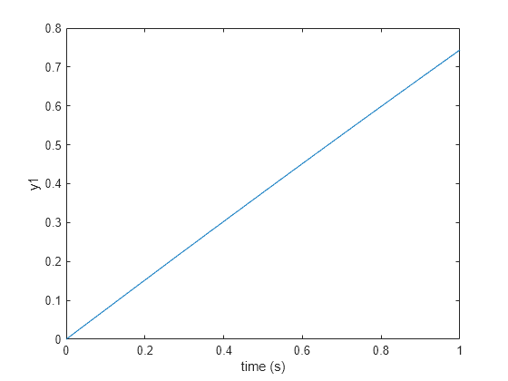
Simulate the model and examine the output response.
m = 1;
out = sim(mdl_step);
t1 = out.logsout{1}.Values.Time;
y1 = out.logsout{1}.Values.Data;
plot(t1,y1);
xlabel("time (s)")
ylabel("y1")
The step response is first-order, thus the order of derivative . You can approximate the critical gain using the slope. For this response, .
b1 = 0.75;
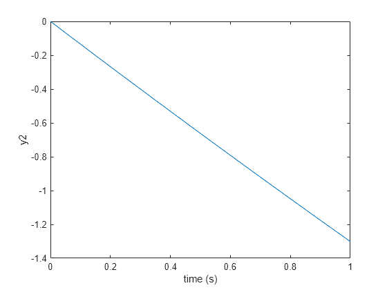
Similarly, specify for the experiment from input to output .
m = 2;
out = sim(mdl_step);
t2 = out.logsout{1}.Values.Time;
y2 = out.logsout{1}.Values.Data;
plot(t2,y2);
xlabel('time (s)')
ylabel('y2')
The step response is also first-order, thus and the critical gain .
b2 = -1.3;
Tune ADRC Controllers
To tune the performance of the ADRC controllers, use the controller bandwidth and observer bandwidth parameters. In this example, the tuning goal is to match the performance of an optimal MPC controller.
Design an MPC controller for the plant model.
Ts = 1; % sample time
mpc1 = mpc(G,Ts);
-->"PredictionHorizon" is empty. Assuming default 10. -->"ControlHorizon" is empty. Assuming default 2. -->"Weights.ManipulatedVariables" is empty. Assuming default 0.00000. -->"Weights.ManipulatedVariablesRate" is empty. Assuming default 0.10000. -->"Weights.OutputVariables" is empty. Assuming default 1.00000.
You can adjust the weights of the controller to tune the performance. For more information, see Tune Weights (Model Predictive Control Toolbox).
Specify weights for the MPC controller.
mpc1.Weights.ManipulatedVariablesRate = 0.7389*[1,1];
mpc1.Weights.OutputVariables = 0.1353*[1,1];
To match the response of the MPC controller, you must set the controller bandwidth and observer bandwidth of the ADRC controllers. For this example, and match the response of the MPC controller.
wc = 0.25;
wo = 3;
Run the model for 45 seconds.
T = 45;
mdl = "ADRCWithBenchmarkMIMO";
open_system(mdl);
sim(mdl);
-->Converting the "Model.Plant" property to state-space.
-->Converting model to discrete time.
-->Integrator added as output disturbance model for measured output #1.
-->Integrator added as output disturbance model for measured output #2.
-->"Model.Noise" is empty. Assuming white noise on each measured output.
View the outputs of the plant using the scope.
open_system(mdl + "/outputs")
The MPC controller and ADRC controllers have a similar response for output . The ADRC controllers have a smaller tracking error for output compared to the MPC controller.
Disturbance Rejection
The model has an external disturbance from 50 to 100 seconds. Run the model to 150 seconds.
T = 150;
sim(mdl);
View the outputs of the plant using the scope.
open_system(mdl + "/outputs")
For this example, the ADRC controllers have better disturbance rejection results compared to the benchmark MPC controller. The outputs more quickly converge to reference values in the presence of a disturbance due to the ADRC controllers using control inputs with larger magnitudes. View the inputs of the plant using the scope.
open_system(mdl + "/inputs")
References
[1] Zheng, Qing, Zhongzhou Chen, and Zhiqiang Gao. “A Dynamic Decoupling Control Approach and Its Applications to Chemical Processes.” In 2007 American Control Conference, 5176–81, 2007. https://doi.org/10.1109/ACC.2007.4282973.
See Also
Active Disturbance Rejection Control