Spatial Contact Force
Model spatial contact between two geometries

Libraries:
Simscape /
Multibody /
Forces and Torques
Description
The Spatial Contact Force block models the contact between a pair of geometries in 3-D space. You can use the built-in penalty method or provide custom normal and friction force laws to model a contact.
Supported Geometries
The Spatial Contact Force block can model contacts between a variety of geometry pairs. You can use the geometries exported from the solid blocks in the Body Elements sublibrary or the geometries of the point and surface blocks in the Curves and Surfaces sublibrary.
All the exported geometries are convex hull representations of the corresponding solids even though some of the solids may have concave shapes. The figure shows the true geometry and convex hull representation of an L-shape solid.
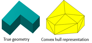
Note that when computing inertial properties, the solid blocks use the true geometry.
The Spatial Contact Force block does not model contacts between certain geometry pairs. This table lists the supported pairs.
| Convex Hull of Solid | Disk | Grid Surface | Infinite Plane | Point | Point Cloud | |
| Convex Hull of Solid | Yes | Yes | No | Yes | Yes | Yes |
| Disk | Yes | No | No | Yes | No | No |
| Grid Surface | No | No | No | No | Yes | Yes |
| Infinite Plane | Yes | Yes | No | No | Yes | Yes |
| Point | Yes | No | Yes | Yes | No | No |
| Point Cloud | Yes | No | Yes | Yes | No | No |
Contact Forces
The image shows how the Spatial Contact Force block models a spatial contact problem between two 3-D geometries. In this case, the contact is between a blue base geometry and a red follower geometry and there is one contact point.

During contact, each geometry has a contact frame. The contact frames are always coincident and located at the contact point. The xy-planes of the contact frames define the contact plane. The z-direction of the contact frames is an outward normal vector for the base geometry, but an inward normal vector for the follower geometry. During continuous contact, the contact frames move around the geometry as the contact point moves.
The block applies contact forces to the geometries at the origin of the contact frames in accordance with Newton's Third Law:
The normal force, , which is aligned with the z-axis of the contact frame. This force pushes the geometries apart in order to reduce penetration.
The frictional force, , which lies in the contact plane. This force opposes the relative tangential velocities between the geometries.
To specify a normal contact force, in the Normal Force section, set
the Method parameter to Smooth Spring-Damper
or Provided by Input. If you select Smooth
Spring-Damper, the normal force is:
,
where:
is the normal force applied in equal-and-opposite fashion to each contacting geometry.
is the penetration depth between two contacting geometries.
is the transition region width specified in the block.
is the first time derivative of the penetration depth.
is the normal-force stiffness specified in the block.
is the normal-force damping specified in the block.
is the smoothing function.
The force law is smoothed near the onset of penetration. When d < w, the smoothing function increases continuously and monotonically over the interval [0, w]. The function is 0 when d = 0, the function is 1 when d = w, and the function has zero derivative with respect to d at the endpoints of the interval.
To better detect contacts when the value of the Transition Region Width parameter is small, the Spatial Contact Force block supports optional zero-crossing detection. The zero-crossing events only occur when the separation distance changes from positive or zero to negative and vice versa.
Note
The zero-crossing detection of the Spatial Contact Force block is different than the zero-crossing detection of other Simulink® blocks, such as From File and Integrator, because the force equation of the Spatial Contact Force is continuous. For more information about zero-crossing detection in Simulink blocks, see Zero-Crossing Detection.
To specify a frictional force, in the Frictional Force section, set
the Method parameter to Smooth Stick-Slip,
Provided by Input, or None. If you
select Smooth Stick-Slip, the frictional force is always directly
opposed to the direction of the relative velocity at the contact point and is related to the
normal force through a coefficient of friction that varies depending on the magnitude of the
relative velocity:
,
where:
is the frictional force.
is the normal force.
is the effective coefficient of friction.
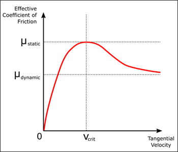
The effective coefficient of friction is a function of the values of the Coefficient of Static Friction, Coefficient of Dynamic Friction, and Critical Velocity parameters, and the magnitude of the relative tangential velocity. At high relative velocities, the value of the effective coefficient of friction is close to that of the coefficient of dynamic friction. At the critical velocity, the effective coefficient of friction achieves a maximum value that is equal to the coefficient of static friction. The graph shows the basic relationship in the typical case where > . In this case, the model is able to approximate stiction with a higher effective coefficient of friction near small tangential velocities.
When modeling contacts that involve a point cloud, the Spatial Contact Force block calculates the contact quantities for each point and the output signals have the same order as the points specified in the Point Could block. For the points that are not in contact with the other geometry, the measured values are zero. When using input forces, the size and order of the input signals must match the size and order of the points specified in the Point Could block.
Examples

Ratchet Lifter
Models a ratchet lifter and demonstrates how to use contact proxies for contact problems that involve complex geometries.

Train Humanoid Walker
Model a humanoid robot using Simscape Multibody™ and train it using either a genetic algorithm (which requires a Global Optimization Toolbox license) or reinforcement learning (which requires Deep Learning Toolbox™ and Reinforcement Learning Toolbox™ licenses).

Using the Reduced Order Flexible Solid Block - Flexible Dipper Arm
Model a flexible dipper arm, such as the arm for an excavator or a backhoe, by using the Reduced Order Flexible Solid block. This block captures the mechanical behavior of a deformable body through reduced-order stiffness and mass matrices that are associated with interface frame locations. In this example, the Partial Differential Equation Toolbox™ is used to create the reduced-order model.

Cable Robot
Models a cable robot. The robot comprises 8 independent belt-cable circuits which control the 6 degrees-of-freedom of the mover. A ball is dropped from a fixed height down the center axis of the mechanism. The mover initially starts directly below the ball and the contact is modeled between the mover and the ball such that the ball bounces elastically when striking the mover. The objective of the mover is to perform increasingly complex maneuvers between successive bounces of the ball. The mover is motion actuated from which the necessary cable, pulley, and motor spool kinematics are computed.
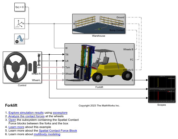
Forklift
Models a forklift which uses the hydraulic and pulley mechanisms to perform the lift action. The tilting of masts is also controlled by hydraulic cylinders. The forklift comprises of 3 masts, namely main mast, top mast and fork mast. The main mast is connected to the chassis by revolute joints and its tilting is governed by the hydraulic tilt cylinders. The top mast slides over the main mast and its motion is governed by the hydraulic lift cylinders. The fork mast slides on the top mast and hangs through belt-cable circuits which drives the movement of the fork mast. A common warehouse application is shown in this example where the objective of the forklift is to grab a box, pass over a bump and place the box in the racks. Spatial Contact Force blocks are used at all contact locations to model the contact between the bodies. The contact between the ground surface and the wheels are modeled using infinite plane block and the contact between the forks and the box are modeled using the point blocks.