Simple Induction Hob Simulation
This example shows how to model a simple induction hob system using Simscape™ Electrical™ libraries. This model focuses on the electromagnetic effect of the winding coils and the eddy current effect in the cooking pot.
Model Overview
Open the model ee_induction_hob.slx.
mdl = "ee_induction_hob";
open_system(mdl)
This example uses blocks from the Simscape Foundation™ and Simscape Electrical libraries. There are two subsystems for the pot and the induction hob.
Open Induction Hob Subsystem
The Induction Hob subsystem represents the electromagnetic portion of the network. To open the subsystem, at the MATLAB® command prompt, enter
open_system('ee_induction_hob/Induction Hob');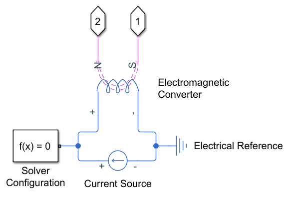
This subsystem contains a Current Source block that models the input current and an Electromagnetic Converter that represents the charging coil inside the inductor and models the electromagnetic induction that converts electrical energy to magnetic energy. The magnetic network is in purple and the electrical network is in dark blue.
Open Pot Subsystem
The Pot subsystem models the cooking pot that contains the fluid you want to heat. To open the subsystem, at the MATLAB command prompt, enter
open_system('ee_induction_hob/Pot');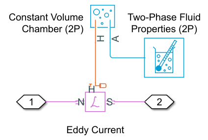
The subsystem contains an Eddy Current block that models the electrical-to-thermal energy conversion, a Constant Volume Chamber (2P) block that models the temperature change in the cooking fluid, and a Two-Phase Fluid Properties block that stores the information of the cooking fluid. The thermal network is in orange and the thermal liquid network is in light blue.
Calculate the Conductance of the Pot
To parameterize the model for different configurations of induction hobs and cooking pots, you must first calculate the conductance of the cooking pot. High frequencies and fast changing fields characterize the system. This means the magnetic field cannot penetrate completely in the inductive material at the bottom of the cooking pot. The penetration depth, , is obtained from this equation:
,
where
is the operating frequency of the input current, in
Hzis the magnetic permeability of the material of the cooking pot, in
H/mis the electrical conductivity of the material of the cooking pot, in
1/(Ωm)
The equivalent resistance, R, and the conductance, G, are independent of the surface area of the cooking pot [1]. For a circular cooking pot, the conductance is equal to
.
In this example, you model an inductor with 15 winding coils that heats a cooking pot made of carbon steel, with a magnetic permeability of and an electrical conductivity of . The Current Source block feeds the winding coils of the inductor with a 10 A and 24 kHz AC current. This example does not model the voltage input from the wall plug or the electrical converters that transform the electrical energy before reaching the inductor.
With these values, the penetration depth is equal to m and the conductance is equal to. Now set the model parameters with these values.
set_param( mdl + "/Induction Hob/Current Source", "ac_current", '10');
set_param( mdl + "/Induction Hob/Current Source", "ac_frequency", '24000');
set_param( mdl + "/Induction Hob/Electromagnetic Converter", "Nw", '15');
set_param( mdl + "/Pot/Eddy Current", "g", '136.55');
Run Simulation
Simulate the model and explore the simulation results in the Simscape Results Explorer window.
result1 = sim(mdl);
sscexplore(result1.simlog)
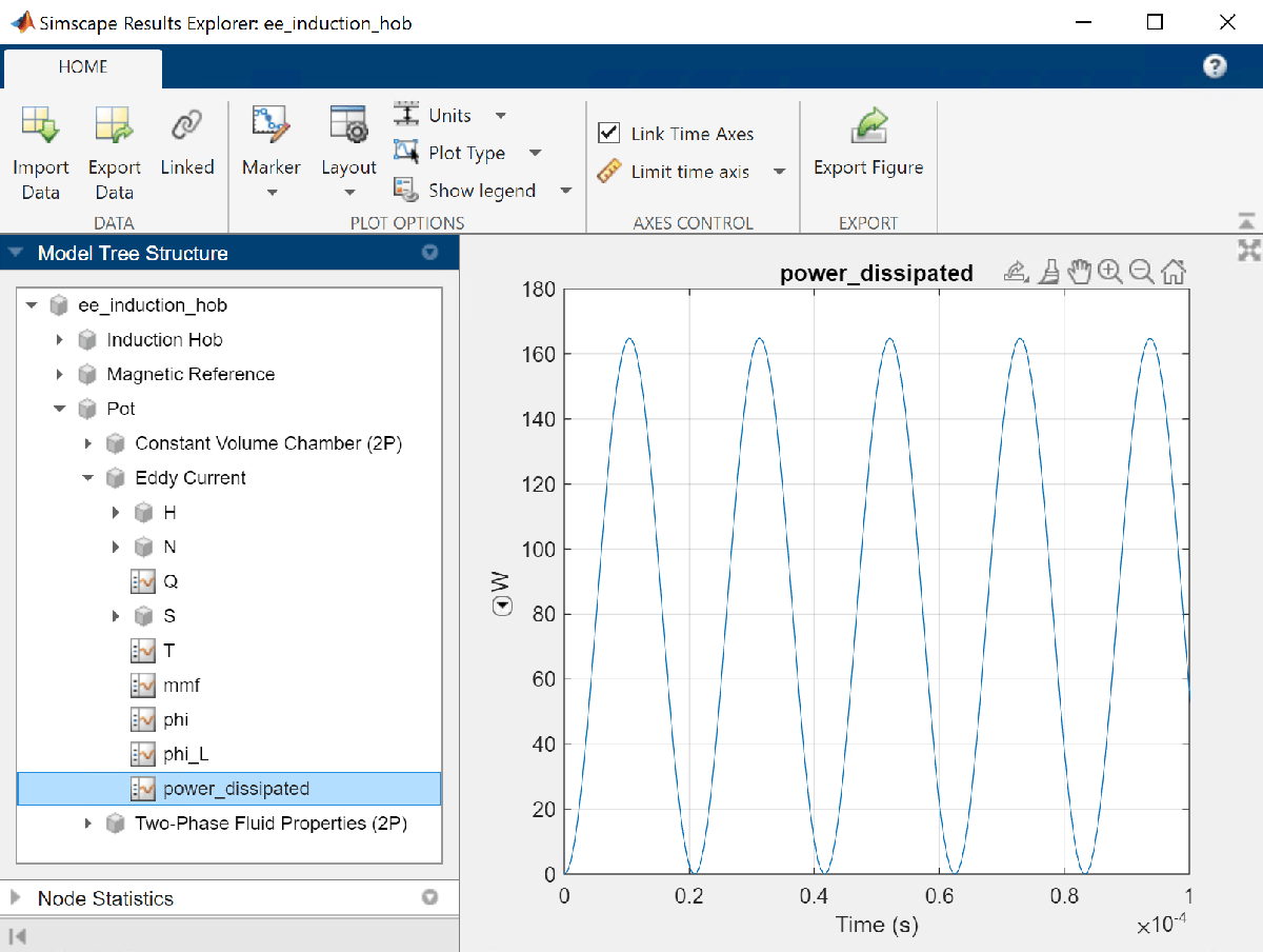
When you click a node in the left pane, the corresponding plots appear in the right pane. For example, check the power output from the Eddy Current block by clicking the power_dissipated variable in Pot > Eddy Current.
Change Parameters for Different Hobs and Cookers
To model different configurations of inductors and cooking pots, modify the parameters of the blocks in the model. For example, to model a different induction hob with 25 winding coils, in the Electromagnetic Converter block, set the Number of winding turns parameter to 25. Then run the simulation again and save the results.
set_param( mdl + "/Induction Hob/Electromagnetic Converter", "Nw", '25');
result2 = sim(mdl);
sscexplore(result2.simlog)
Now model a cooking pot made of gray cast iron, with a magnetic permeability of and an electrical conductivity of . With these values, the conductance is equal to . In the Eddy Current block, set the Conductance of eddy current loop parameter to 29.13. Again, run the simulation and save the new results.
set_param( mdl + "/Pot/Eddy Current", "g", '29.13');
result3 = sim(mdl);
sscexplore(result3.simlog)
Plot and Compare the Results
To extract, plot, and compare the results of the previous simulations, at the MATLAB Command Window, enter:
figure
hold on
yline(mean(result1.simlog.Pot.Eddy_Current.power_dissipated.series.values), "b")
yline(mean(result2.simlog.Pot.Eddy_Current.power_dissipated.series.values), "k")
yline(mean(result3.simlog.Pot.Eddy_Current.power_dissipated.series.values), "r")
simTime = result1.simlog.Pot.Constant_Volume_Chamber_2P.T_I.series.time;
xlim([0, simTime(end)])
xlabel("Time [s]")
ylabel("Power [W]")
title("Averaged Power Dissipated from Eddy Current")
legend("Carbon Steel, 15 Winding", "Carbon Steel, 25 Winding", "Cast Iron, 25 Winding", "Location", "best")
![Figure contains an axes object. The axes object with title Averaged Power Dissipated from Eddy Current, xlabel Time [s], ylabel Power [W] contains 3 objects of type constantline. These objects represent Carbon Steel, 15 Winding, Carbon Steel, 25 Winding, Cast Iron, 25 Winding.](../../examples/simscapeelectrical/win64/InductionHobExample_05.png)
The first plot shows the averaged power dissipated from the Eddy Current block for each of the three cooking pots. The carbon steel cooking pot with 25 winding coils transforms more power into thermal than the carbon steel cooking pot with 15 winding coils. With the same number of winding coils, the cast iron pot has more cooking power due to its much lower conductance.
figure
hold on
plot(result1.simlog.Pot.Constant_Volume_Chamber_2P.T_I.series.time, result1.simlog.Pot.Constant_Volume_Chamber_2P.T_I.series.values - 273.15, "b")
plot(result2.simlog.Pot.Constant_Volume_Chamber_2P.T_I.series.time, result2.simlog.Pot.Constant_Volume_Chamber_2P.T_I.series.values - 273.15, "k")
plot(result3.simlog.Pot.Constant_Volume_Chamber_2P.T_I.series.time, result3.simlog.Pot.Constant_Volume_Chamber_2P.T_I.series.values - 273.15, "r")
xlabel("Time [s]")
ylabel("Temperature [Celsius]")
title("Temperature of the Pot")
legend("Carbon Steel, 15 Winding", "Carbon Steel, 25 Winding", "Cast Iron, 25 Winding", "Location", "best")
![Figure contains an axes object. The axes object with title Temperature of the Pot, xlabel Time [s], ylabel Temperature [Celsius] contains 3 objects of type line. These objects represent Carbon Steel, 15 Winding, Carbon Steel, 25 Winding, Cast Iron, 25 Winding.](../../examples/simscapeelectrical/win64/InductionHobExample_06.png)
The second plot compares the temperature rise for the three cooking pots. Similarly to the results of the first plot, a higher number of winding coils and a low-conductance material provide more power and quicker temperature rise.
Reference
[1] Siakavellas, N. J. "Two simple models for analytical calculation of eddy currents in thin conducting plates," in IEEE Transactions on Magnetics, vol. 33, no. 3, pp. 2245-2257.