Cluster Gaussian Mixture Data Using Hard Clustering
This example shows how to implement hard clustering on simulated data from a mixture of Gaussian distributions.
Gaussian mixture models can be used for clustering data, by realizing that the multivariate normal components of the fitted model can represent clusters.
Simulate Data from a Mixture of Gaussian Distributions
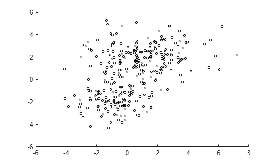
Simulate data from a mixture of two bivariate Gaussian distributions using mvnrnd.
rng('default')  % For reproducibility
mu1 = [1 2];
sigma1 = [3 .2; .2 2];
mu2 = [-1 -2];
sigma2 = [2 0; 0 1];
X = [mvnrnd(mu1,sigma1,200); mvnrnd(mu2,sigma2,100)];
n = size(X,1);

figure
scatter(X(:,1),X(:,2),10,'ko')
Fit a Gaussian Mixture Model to the Simulated Data
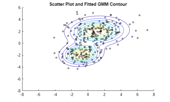
Fit a two-component Gaussian mixture model (GMM). Here, you know the correct number of components to use. In practice, with real data, this decision would require comparing models with different numbers of components. Also, request to display the final iteration of the expectation-maximization fitting routine.
options = statset('Display','final');
gm = fitgmdist(X,2,'Options',options)
26 iterations, log-likelihood = -1210.59

gm =

Gaussian mixture distribution with 2 components in 2 dimensions
Component 1:
Mixing proportion: 0.629514
Mean:    1.0756    2.0421

Component 2:
Mixing proportion: 0.370486
Mean:   -0.8296   -1.8488
Plot the estimated probability density contours for the two-component mixture distribution. The two bivariate normal components overlap, but their peaks are distinct. This suggests that the data could reasonably be divided into two clusters.
hold on
gmPDF = @(x,y) arrayfun(@(x0,y0) pdf(gm,[x0,y0]),x,y);
fcontour(gmPDF,[-8,6])
title('Scatter Plot and Fitted GMM Contour')
hold off
Cluster the Data Using the Fitted GMM
cluster implements "hard clustering", a method that assigns each data point to exactly one cluster. For GMM, cluster assigns each point to one of the two mixture components in the GMM. The center of each cluster is the corresponding mixture component mean. For details on "soft clustering," see Cluster Gaussian Mixture Data Using Soft Clustering.
Partition the data into clusters by passing the fitted GMM and the data to cluster.
idx = cluster(gm,X);
cluster1 = (idx == 1); % |1| for cluster 1 membership
cluster2 = (idx == 2); % |2| for cluster 2 membership

figure
gscatter(X(:,1),X(:,2),idx,'rb','+o')
legend('Cluster 1','Cluster 2','Location','best')
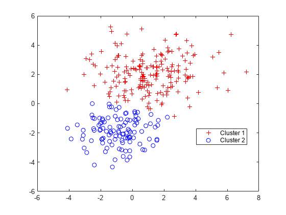
Each cluster corresponds to one of the bivariate normal components in the mixture distribution. cluster assigns data to clusters based on a cluster membership score. Each cluster membership scores is the estimated posterior probability that the data point came from the corresponding component. cluster assigns each point to the mixture component corresponding to the highest posterior probability.
You can estimate cluster membership posterior probabilities by passing the fitted GMM and data to either:
cluster, and request to return the third output argument
Estimate Cluster Membership Posterior Probabilities
Estimate and plot the posterior probability of the first component for each point.
P = posterior(gm,X);

figure
scatter(X(cluster1,1),X(cluster1,2),10,P(cluster1,1),'+')
hold on
scatter(X(cluster2,1),X(cluster2,2),10,P(cluster2,1),'o')
hold off
clrmap = jet(80);
colormap(clrmap(9:72,:))
ylabel(colorbar,'Component 1 Posterior Probability')
legend('Cluster 1','Cluster 2','Location','best')
title('Scatter Plot and Cluster 1 Posterior Probabilities')
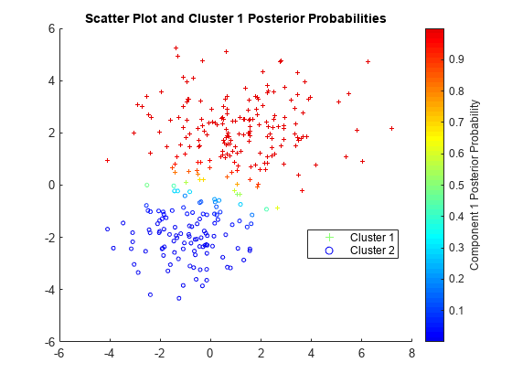
P is an n-by-2 matrix of cluster membership posterior probabilities. The first column contains the probabilities for cluster 1 and the second column corresponds to cluster 2.
Assign New Data to Clusters
You can also use the cluster method to assign new data points to the mixture components found in the original data.
Simulate new data from a mixture of Gaussian distributions. Rather than using mvnrnd, you can create a GMM with the true mixture component means and standard deviations using gmdistribution, and then pass the GMM to random to simulate data.
Mu = [mu1; mu2];
Sigma = cat(3,sigma1,sigma2);
p = [0.75 0.25]; % Mixing proportions

gmTrue = gmdistribution(Mu,Sigma,p);
X0 = random(gmTrue,75);
Assign clusters to the new data by pass the fitted GMM (gm) and the new data to cluster. Request cluster membership posterior probabilities.
[idx0,~,P0] = cluster(gm,X0);

figure
fcontour(gmPDF,[min(X0(:,1)) max(X0(:,1)) min(X0(:,2)) max(X0(:,2))])
hold on
gscatter(X0(:,1),X0(:,2),idx0,'rb','+o')
legend('Fitted GMM Contour','Cluster 1','Cluster 2','Location','best')
title('New Data Cluster Assignments')
hold off
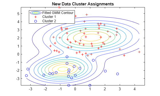
For cluster to provide meaningful results when clustering new data, X0 should come from the same population as X, the original data used to create the mixture distribution. In particular, when computing the posterior probabilities for X0, cluster and posterior use the estimated mixing probabilities.
See Also
fitgmdist | gmdistribution | cluster | posterior | random