Cluster Gaussian Mixture Data Using Soft Clustering
This example shows how to implement soft clustering on simulated data from a mixture of Gaussian distributions.
cluster estimates cluster membership posterior probabilities, and then assigns each point to the cluster corresponding to the maximum posterior probability. Soft clustering is an alternative clustering method that allows some data points to belong to multiple clusters. To implement soft clustering:
Assign a cluster membership score to each data point that describes how similar each point is to each cluster's archetype. For a mixture of Gaussian distributions, the cluster archetype is corresponding component mean, and the component can be the estimated cluster membership posterior probability.
Rank the points by their cluster membership score.
Inspect the scores and determine cluster memberships.
For algorithms that use posterior probabilities as scores, a data point is a member of the cluster corresponding to the maximum posterior probability. However, if there are other clusters with corresponding posterior probabilities that are close to the maximum, then the data point can also be a member of those clusters. It is good practice to determine the threshold on scores that yield multiple cluster memberships before clustering.
This example follows from Cluster Gaussian Mixture Data Using Hard Clustering.
Simulate data from a mixture of two bivariate Gaussian distributions.
rng(0,'twister')  % For reproducibility
mu1 = [1 2];
sigma1 = [3 .2; .2 2];
mu2 = [-1 -2];
sigma2 = [2 0; 0 1];
X = [mvnrnd(mu1,sigma1,200); mvnrnd(mu2,sigma2,100)];
Fit a two-component Gaussian mixture model (GMM). Because there are two components, suppose that any data point with cluster membership posterior probabilities in the interval [0.4,0.6] can be a member of both clusters.
gm = fitgmdist(X,2);
threshold = [0.4 0.6];
Estimate component-member posterior probabilities for all data points using the fitted GMM gm. These represent cluster membership scores.
P = posterior(gm,X);
For each cluster, rank the membership scores for all data points. For each cluster, plot each data points membership score with respect to its ranking relative to all other data points.
n = size(X,1);
[~,order] = sort(P(:,1));

figure
plot(1:n,P(order,1),'r-',1:n,P(order,2),'b-')
legend({'Cluster 1', 'Cluster 2'})
ylabel('Cluster Membership Score')
xlabel('Point Ranking')
title('GMM with Full Unshared Covariances')
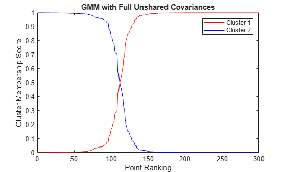
Although a clear separation is hard to see in a scatter plot of the data, plotting the membership scores indicates that the fitted distribution does a good job of separating the data into groups.
Plot the data and assign clusters by maximum posterior probability. Identify points that could be in either cluster.
idx = cluster(gm,X);
idxBoth = find(P(:,1)>=threshold(1) & P(:,1)<=threshold(2));
numInBoth = numel(idxBoth)
numInBoth =
7
figure
gscatter(X(:,1),X(:,2),idx,'rb','+o',5)
hold on
plot(X(idxBoth,1),X(idxBoth,2),'ko','MarkerSize',10)
legend({'Cluster 1','Cluster 2','Both Clusters'},'Location','SouthEast')
title('Scatter Plot - GMM with Full Unshared Covariances')
hold off
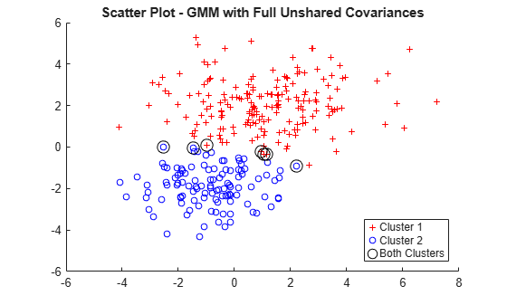
Using the score threshold interval, seven data points can be in either cluster.
Soft clustering using a GMM is similar to fuzzy k-means clustering, which also assigns each point to each cluster with a membership score. The fuzzy k-means algorithm assumes that clusters are roughly spherical in shape, and all of roughly equal size. This is comparable to a Gaussian mixture distribution with a single covariance matrix that is shared across all components, and is a multiple of the identity matrix. In contrast, gmdistribution allows you to specify different covariance structures. The default is to estimate a separate, unconstrained covariance matrix for each component. A more restricted option, closer to k-means, is to estimate a shared, diagonal covariance matrix.
Fit a GMM to the data, but specify that the components share the same, diagonal covariance matrix. This specification is similar to implementing fuzzy k-means clustering, but provides more flexibility by allowing unequal variances for different variables.
gmSharedDiag = fitgmdist(X,2,'CovType','Diagonal', ...
    'SharedCovariance',true');
Estimate component-member posterior probabilities for all data points using the fitted GMM gmSharedDiag. Estimate soft cluster assignments.
[idxSharedDiag,~,PSharedDiag] = cluster(gmSharedDiag,X);
idxBothSharedDiag = find(PSharedDiag(:,1)>=threshold(1) & ...
PSharedDiag(:,1)<=threshold(2));
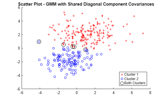
numInBoth = numel(idxBothSharedDiag)numInBoth = 5
Assuming shared, diagonal covariances among components, five data points could be in either cluster.
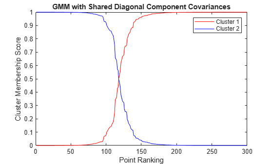
For each cluster:
Rank the membership scores for all data points.
Plot each data points membership score with respect to its ranking relative to all other data points.
[~,orderSharedDiag] = sort(PSharedDiag(:,1));

figure
plot(1:n,PSharedDiag(orderSharedDiag,1),'r-',...
    1:n,PSharedDiag(orderSharedDiag,2),'b-')
legend({'Cluster 1' 'Cluster 2'},'Location','NorthEast')
ylabel('Cluster Membership Score')
xlabel('Point Ranking')
title('GMM with Shared Diagonal Component Covariances')
Plot the data and identify the hard, clustering assignments from the GMM analysis assuming the shared, diagonal covariances among components. Also, identify those data points that could be in either cluster.
figure
gscatter(X(:,1),X(:,2),idxSharedDiag,'rb','+o',5)
hold on
plot(X(idxBothSharedDiag,1),X(idxBothSharedDiag,2),'ko','MarkerSize',10)
legend({'Cluster 1','Cluster 2','Both Clusters'},'Location','SouthEast')
title('Scatter Plot - GMM with Shared Diagonal Component Covariances')
hold off
See Also
fitgmdist | gmdistribution | cluster