Main Content

predict

Predict response of Gaussian process regression model

Syntax

ypred = predict(gprMdl,Xnew)
[ypred,ysd,yint] = predict(gprMdl,Xnew)
[ypred,ysd,yint] = predict(gprMdl,Xnew,Name,Value)

Description

ypred = predict(gprMdl,Xnew) returns the predicted responses ypred for the Gaussian process regression (GPR) model gprMdl and the predictor values in Xnew.

[ypred,ysd,yint] = predict(gprMdl,Xnew) also returns the standard deviations ysd and 95% prediction intervals yint of the response variable, evaluated at each observation in Xnew using the trained GPR model.

[ypred,ysd,yint] = predict(gprMdl,Xnew,Name,Value) specifies additional options using one or more name-value arguments. For example, specify the significance level for the confidence level of the prediction intervals yint.

Input Arguments

expand all

Gaussian process regression model, specified as a RegressionGP (full) or CompactRegressionGP (compact) object.

New values for the predictors that fitrgp uses in training the GPR model, specified as a table or an m-by-d matrix. m is the number of observations and d is the number of predictor variables in the training data.

If you trained gprMdl on a table, then Xnew must be a table that contains all the predictor variables used to train gprMdl.

If you trained gprMdl on a matrix, then Xnew must be a numeric matrix with d columns.

Data Types: single | double | table

Name-Value Arguments

Specify optional pairs of arguments as Name1=Value1,...,NameN=ValueN, where Name is the argument name and Value is the corresponding value. Name-value arguments must appear after other arguments, but the order of the pairs does not matter.

Before R2021a, use commas to separate each name and value, and enclose Name in quotes.

Example: predict(grpMdl,Xnew,"Alpha",0.1) specifies the confidence level of the prediction intervals to be 90%.

Significance level for the confidence level of the prediction intervals yint, specified as a numeric scalar in the range [0,1]. The confidence level of yint is equal to 100(1 – Alpha)%.

Example: 'Alpha',0.01 specifies to return 99% prediction intervals.

Data Types: single | double

Since R2023b

Predicted response value to use for observations with missing predictor values, specified as "median", "mean", or a numeric scalar.

ValueDescription
"median"predict uses the median of the observed response values in the training data as the predicted response value for observations with missing predictor values.
"mean"predict uses the mean of the observed response values in the training data as the predicted response value for observations with missing predictor values.
Numeric scalarpredict uses this value as the predicted response value for observations with missing predictor values.

Example: "PredictionForMissingValue","mean"

Example: "PredictionForMissingValue",NaN

Data Types: single | double | char | string

Output Arguments

expand all

Predicted responses, returned as a column vector of length n, where n is the number of observations in the predictor data Xnew.

Standard deviations of the response variable, evaluated at each observation in the predictor data Xnew, returned as a column vector of length n, where n is the number of observations in Xnew. The ith element ysd(i) contains the standard deviation of the ith response for the ith observation Xnew(i,:), estimated using the trained GPR model gprMdl.

Prediction intervals of the response variable, evaluated at each observation in the predictor data Xnew, returned as an n-by-2 matrix, where n is the number of observations in Xnew. The ith row yint(i,:) contains the 100(1 – Alpha)% prediction interval of the ith response for the ith observation Xnew(i,:). The Alpha value is the probability that the prediction interval does not contain the true response value for Xnew(i,:). The first column of yint contains the lower limits of the prediction intervals, and the second column contains the upper limits.

Examples

expand all

Generate the sample data.

n = 10000;
rng(1) % For reproducibility
x = linspace(0.5,2.5,n)';
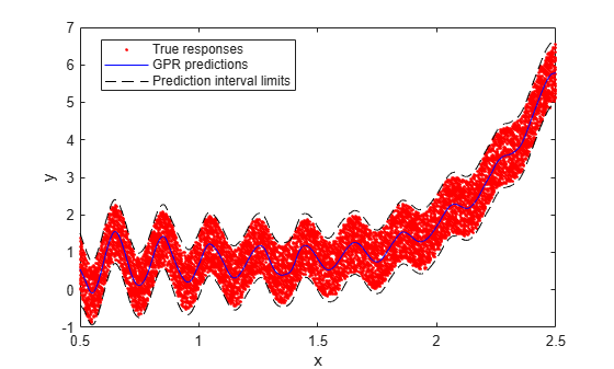
y = sin(10*pi.*x) ./ (2.*x)+(x-1).^4 + 1.5*rand(n,1);

Fit a GPR model using the Matern 3/2 kernel function with separate length scale for each predictor and an active set size of 100. Use the subset of regressors approximation method for parameter estimation and fully independent conditional method for prediction.

gprMdl = fitrgp(x,y,'KernelFunction','ardmatern32', ...
    'ActiveSetSize',100,'FitMethod','sr','PredictMethod','fic');

Compute the predictions.

[ypred,~,yci] = predict(gprMdl,x);

Plot the data along with the predictions and prediction intervals.

plot(x,y,'r.')
hold on
plot(x,ypred,'b-')
plot(x,yci(:,1),'k--')
plot(x,yci(:,2),'k--')
xlabel('x')
ylabel('y')
legend('True responses','GPR predictions', ...
    'Prediction interval limits','Location','best')

Figure contains an axes object. The axes object with xlabel x, ylabel y contains 4 objects of type line. One or more of the lines displays its values using only markers These objects represent True responses, GPR predictions, Prediction interval limits.

Load the sample data and store in a table.

load fisheriris
tbl = table(meas(:,1),meas(:,2),meas(:,3),meas(:,4),species,...
'VariableNames',{'meas1','meas2','meas3','meas4','species'});

Fit a GPR model using the first measurement as the response and the other variables as the predictors.
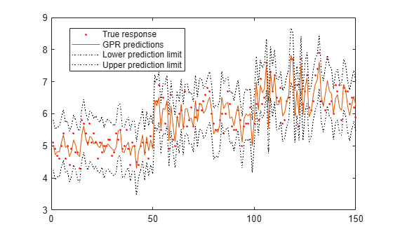
mdl = fitrgp(tbl,'meas1');

Compute the predictions and the 99% confidence intervals.

[ypred,~,yci] = predict(mdl,tbl,'Alpha',0.01);

Plot the true response and the predictions along with the prediction intervals.

figure();
plot(mdl.Y,'r.');
hold on;
plot(ypred);
plot(yci(:,1),'k:');
plot(yci(:,2),'k:');
legend('True response','GPR predictions',...
'Lower prediction limit','Upper prediction limit',...
'Location','Best');

Figure contains an axes object. The axes object contains 4 objects of type line. One or more of the lines displays its values using only markers These objects represent True response, GPR predictions, Lower prediction limit, Upper prediction limit.

Load the sample data.
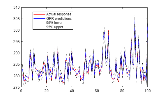
load('gprdata.mat');

The data contains training and test data. There are 500 observations in training data and 100 observations in test data. The data has 6 predictor variables. This is simulated data.

Fit a GPR model using the squared exponential kernel function with a separate length scale for each predictor. Standardize predictors in the training data. Use the exact fitting and prediction methods.

gprMdl = fitrgp(Xtrain,ytrain,'Basis','constant',...
'FitMethod','exact','PredictMethod','exact',...
'KernelFunction','ardsquaredexponential','Standardize',1);

Predict the responses for test data.

[ytestpred,~,ytestci] = predict(gprMdl,Xtest);

Plot the test response along with the predictions.

figure;
plot(ytest,'r');
hold on;
plot(ytestpred,'b');
plot(ytestci(:,1),'k:');
plot(ytestci(:,2),'k:');
legend('Actual response','GPR predictions',...
'95% lower','95% upper','Location','Best');
hold off

Figure contains an axes object. The axes object contains 4 objects of type line. These objects represent Actual response, GPR predictions, 95% lower, 95% upper.

Tips

  • You can choose the prediction method while training the GPR model using the PredictMethod name-value pair argument in fitrgp. The default prediction method is 'exact' for n ≤ 10000, where n is the number of observations in the training data, and 'bcd' (block coordinate descent), otherwise.

  • Computation of standard deviations, ysd, and prediction intervals, yint, is not supported when PredictMethod is 'bcd'.

  • If gprMdl is a CompactRegressionGP object, you cannot compute standard deviations, ysd, or prediction intervals, yint, for PredictMethod equal to 'sr' or 'fic'. To compute ysd and yint for PredictMethod equal to 'sr' or 'fic', use the full regression (RegressionGP) object.

Alternatives

You can use resubPredict to compute the predicted responses for the trained GPR model at the observations in the training data.

Simulink Block

To integrate the prediction of a Gaussian process regression model into Simulink®, you can use the RegressionGP Predict block in the Statistics and Machine Learning Toolbox™ library or a MATLAB® Function block with the predict function. For examples, see Predict Responses Using RegressionGP Predict Block and Predict Class Labels Using MATLAB Function Block.

When deciding which approach to use, consider the following:

  • If you use the Statistics and Machine Learning Toolbox library block, you can use the Fixed-Point Tool (Fixed-Point Designer) to convert a floating-point model to fixed point.

  • Support for variable-size arrays must be enabled for a MATLAB Function block with the predict function.

  • If you use a MATLAB Function block, you can use MATLAB functions for preprocessing or post-processing before or after predictions in the same MATLAB Function block.

Extended Capabilities

Version History

Introduced in R2015b

expand all