predict

Class: FeatureSelectionNCARegression

Predict responses using neighborhood component analysis (NCA) regression model

Syntax

ypred = predict(mdl,X)


Description

ypred = predict(mdl,X) computes the predicted response values, ypred, corresponding to rows of X, using the model mdl.

Input Arguments

mdl — Neighborhood component analysis model for regression

FeatureSelectionNCARegression object

Neighborhood component analysis model for regression, specified as a FeatureSelectionNCARegression object.

X — Predictor variable values

n-by-p matrix

Predictor variable values, specified as an n-by-p matrix, where n is the number of observations and p is the number of predictor variables.

Data Types: single | double

Output Arguments

ypred — Predicted response values

n-by-1 vector

Predicted response values, specified as an n-by-1 vector, where n is the number of observations.

Examples

Tune NCA Model for Regression Using loss and predict

Load the sample data.

Download the housing data [1], from the UCI Machine Learning Repository [2]. The dataset has 506 observations. The first 13 columns contain the predictor values and the last column contains the response values. The goal is to predict the median value of owner-occupied homes in suburban Boston as a function of 13 predictors.

Load the data and define the response vector and the predictor matrix.

load('housing.data');
X = housing(:,1:13);
y = housing(:,end);

Divide the data into training and test sets using the 4th predictor as the grouping variable for a stratified partitioning. This ensures that each partition includes similar amount of observations from each group.

rng(1) % For reproducibility
cvp = cvpartition(X(:,4),'Holdout',56);
Xtrain = X(cvp.training,:);
ytrain = y(cvp.training,:);
Xtest  = X(cvp.test,:);
ytest  = y(cvp.test,:);

cvpartition randomly assigns 56 observations into a test set and the rest of the data into a training set.

Perform Feature Selection Using Default Settings

Perform feature selection using NCA model for regression. Standardize the predictor values.

nca = fsrnca(Xtrain,ytrain,'Standardize',1);

Plot the feature weights.

figure()
plot(nca.FeatureWeights,'ro')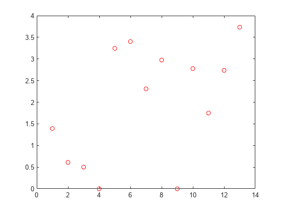

The weights of irrelevant features are expected to approach zero. fsrnca identifies two features as irrelevant.

Compute the regression loss.

L = loss(nca,Xtest,ytest,'LossFunction','mad')

L = 2.5394

Compute the predicted response values for the test set and plot them versus the actual response.

ypred = predict(nca,Xtest);
figure()
plot(ypred,ytest,'bo')
xlabel('Predicted response')
ylabel('Actual response')

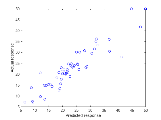
A perfect fit versus the actual values forms a 45 degree straight line. In this plot, the predicted and actual response values seem to be scattered around this line. Tuning $$\lambda$$ (regularization parameter) value usually helps improve the performance.

Tune the regularization parameter using 10-fold cross-validation

Tuning $$\lambda$$ means finding the $$\lambda$$ value that will produce the minimum regression loss. Here are the steps for tuning $$\lambda$$ using 10-fold cross-validation:

1. First partition the data into 10 folds. For each fold, cvpartition assigns 1/10th of the data as a training set, and 9/10th of the data as a test set.

n = length(ytrain);
cvp = cvpartition(Xtrain(:,4),'kfold',10);
numvalidsets = cvp.NumTestSets;

Assign the $$\lambda$$ values for the search. Create an array to store the loss values.

lambdavals = linspace(0,2,30)*std(ytrain)/n;
lossvals = zeros(length(lambdavals),numvalidsets);

2. Train the neighborhood component analysis (nca) model for each $$\lambda$$ value using the training set in each fold.

3. Fit a Gaussian process regression (gpr) model using the selected features. Next, compute the regression loss for the corresponding test set in the fold using the gpr model. Record the loss value.

4. Repeat this for each $$\lambda$$ value and each fold.

 for i = 1:length(lambdavals)
    for k = 1:numvalidsets
        X = Xtrain(cvp.training(k),:);
        y = ytrain(cvp.training(k),:);
        Xvalid  = Xtrain(cvp.test(k),:);
        yvalid  = ytrain(cvp.test(k),:);

        nca = fsrnca(X,y,'FitMethod','exact',...
             'Lambda',lambdavals(i),...
             'Standardize',1,'LossFunction','mad');

        % Select features using the feature weights and a relative
        % threshold.
        tol    = 1e-3;
        selidx = nca.FeatureWeights > tol*max(1,max(nca.FeatureWeights));

        % Fit a non-ARD GPR model using selected features.
        gpr = fitrgp(X(:,selidx),y,'Standardize',1,...
              'KernelFunction','squaredexponential','Verbose',0);


        lossvals(i,k) = loss(gpr,Xvalid(:,selidx),yvalid);

    end
 end

Compute the average loss obtained from the folds for each $$\lambda$$ value. Plot the mean loss versus the $$\lambda$$ values.

meanloss = mean(lossvals,2);
figure;
plot(lambdavals,meanloss,'ro-');
xlabel('Lambda');
ylabel('Loss (MSE)');
grid on;

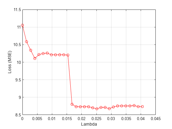
Find the $$\lambda$$ value that produces the minimum loss value.

[~,idx] = min(meanloss);
bestlambda = lambdavals(idx)

bestlambda = 0.0251

Perform feature selection for regression using the best $$\lambda$$ value. Standardize the predictor values.

nca2 = fsrnca(Xtrain,ytrain,'Standardize',1,'Lambda',bestlambda,...
    'LossFunction','mad');

Plot the feature weights.

figure()
plot(nca.FeatureWeights,'ro')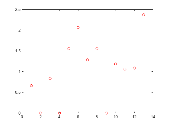

Compute the loss using the new nca model on the test data, which is not used to select the features.

L2 = loss(nca2,Xtest,ytest,'LossFunction','mad')

L2 = 2.0560

Tuning the regularization parameter helps identify the relevant features and reduces the loss.

Plot the predicted versus the actual response values in the test set.

ypred = predict(nca2,Xtest);
figure;
plot(ypred,ytest,'bo');

The predicted response values seem to be closer to the actual values as well.

References

[1] Harrison, D. and D.L., Rubinfeld. "Hedonic prices and the demand for clean air." J. Environ. Economics & Management. Vol.5, 1978, pp. 81-102.

[2] Lichman, M. UCI Machine Learning Repository, Irvine, CA: University of California, School of Information and Computer Science, 2013. https://archive.ics.uci.edu/ml.

Version History

Introduced in R2016b