loss
Regression or classification error of incremental drift-aware learner
Since R2022b
Description
Err = loss(Mdl,X,Y,Name=Value)
Examples
Load the human activity dataset. Randomly shuffle the data.
load humanactivity;
n = numel(actid);
rng(123) % For reproducibility
idx = randsample(n,n);
For details on the data set, enter Description at the command line.
Define the predictor and response variables.
X = feat(idx,:);
Y = actid(idx);
Responses can be one of five classes: Sitting, Standing, Walking, Running, or Dancing.
Dichotomize the response by identifying whether the subject is moving (actid > 2).
Y = Y > 2;
Flip labels for the second half of the dataset to simulate drift.
Y(floor(numel(Y)/2):end,:) = ~Y(floor(numel(Y)/2):end,:);
Initiate a default incremental drift-aware model for classification as follows:
Create a default incremental linear SVM model for binary classification.
Initiate a default incremental drift-aware model using the incremental linear SVM model as the base learner.
BaseLearner = incrementalClassificationLinear();
idaMdl = incrementalDriftAwareLearner(BaseLearner);
idaMdl is an incrementalDriftAwareLearner model. All its properties are read-only.
Preallocate the number of variables in each chunk for creating a stream of data and the variable to store the classification error.
numObsPerChunk = 50;
nchunk = floor(n/numObsPerChunk);
ce = array2table(zeros(nchunk,3),VariableNames=["Cumulative" "Window" "Loss"]);
PoL = zeros(nchunk,numObsPerChunk); % To store per observation loss values
driftTimes = [];
Simulate a data stream with incoming chunks of 50 observations each. At each iteration:
Call
updateMetricsto measure the cumulative performance and the performance within a window of observations. Overwrite the previous incremental model with a new one to track performance metrics.Call
fitto fit the model to the incoming chunk. Overwrite the previous incremental model with a new one fitted to the incoming observations.Call
perObservationLossto compute classification error on each observation in the incoming chunk of data.Call
lossto measure the model performance on the incoming chunk.Store all performance metrics in
ceto see how they evolve during incremental learning. TheMetricsproperty ofidaMdlstores the cumulative and window classification error, which is updated at each iteration. Store the loss values for each chunk in the third column ofce.
for j = 1:nchunk

 ibegin = min(n,numObsPerChunk*(j-1)+1);
 iend   = min(n,numObsPerChunk*j);
 idx = ibegin:iend;

 idaMdl = updateMetrics(idaMdl,X(idx,:),Y(idx));
 idaMdl = fit(idaMdl,X(idx,:),Y(idx));

 PoL(j,:) = perObservationLoss(idaMdl,X(idx,:),Y(idx));
 ce{j,["Cumulative" "Window"]} = idaMdl.Metrics{"ClassificationError",:};
 ce{j,"Loss"} = loss(idaMdl,X(idx,:),Y(idx));
 if idaMdl.DriftDetected
    driftTimes(end+1) = j;
 end
end
The updateMetrics function evaluates the performance of the model as it processes incoming observations. The function writes specified metrics, measured cumulatively and within a specified window of processed observations, to the Metrics model property. The fit function fits the model by updating the base learner and monitoring for drift given an incoming batch of data.
Plot the cumulative and per window classification error. Mark the warmup and training periods, and where the drift was introduced.
h = plot(ce.Variables);
xlim([0 nchunk])
ylim([0 0.07])
ylabel("Classification Error")
xlabel("Iteration")

xline(idaMdl.MetricsWarmupPeriod/numObsPerChunk,"g-.","Warmup Period",LineWidth= 1.5)
xline(idaMdl.TrainingPeriod/numObsPerChunk,"b-.","Training Period",LabelVerticalAlignment="middle",LineWidth= 1.5)
%xline(floor(numel(Y)/2)/numObsPerChunk,"m--","Drift",LabelVerticalAlignment="middle",LineWidth= 1.5)

xline(driftTimes,"m--","Drift",LabelVerticalAlignment="middle",LineWidth=1.5)
legend(h,ce.Properties.VariableNames)
legend(h,Location="best")
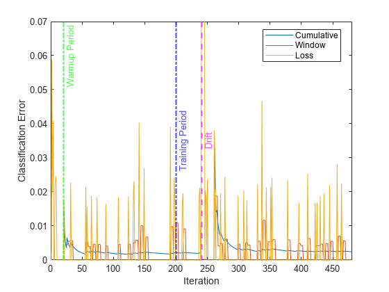
The yellow line represents the classification error on each incoming chunk of data. loss is agnostic of the metrics warm-up period, so it measures the classification error for all iterations. After the metrics warm-up period, idaMdl tracks the cumulative and window metrics.
Plot the per observation loss.
figure()
plot(PoL,'b.');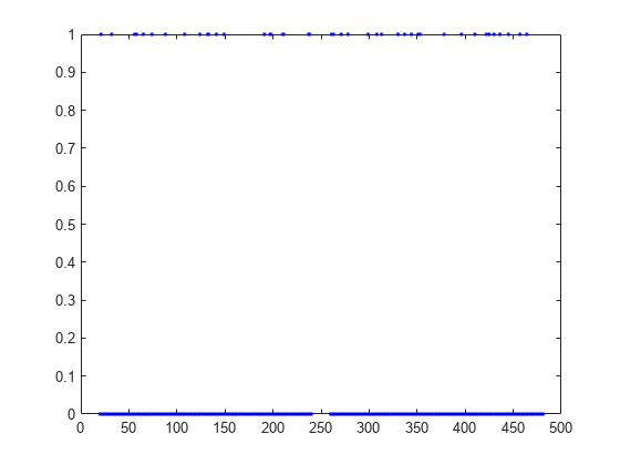
perObservationLoss computes the classification loss for each observation in the incoming chunk of data.
Create the random concept data and the concept drift generator using the helper functions HelperRegrGenerator and HelperConceptDriftGenerator, respectively.
concept1 = HelperRegrGenerator(NumFeatures=100,NonZeroFeatures=[1,20,40,50,55], ...
        FeatureCoefficients=[4,5,10,-2,-6],NoiseStd=1.1);
concept2 = HelperRegrGenerator(NumFeatures=100,NonZeroFeatures=[1,20,40,50,55], ...
        FeatureCoefficients=[4,7,10,-1,-5],NoiseStd=1.1);
driftGenerator = HelperConceptDriftGenerator(concept1,concept2,15000,1250);
HelperRegrGenerator generates streaming data using features and feature coefficients for regression specified in the call to the function. At each step, the function samples the predictors from a normal distribution. Then, it computes the response using the feature coefficients and predictor values and adding a random noise from a normal distribution with mean zero and specified noise standard deviation.
HelperConceptDriftGenerator establishes the concept drift. The object uses a sigmoid function 1./(1+exp(-4*(numobservations-position)./width)) to decide the probability of choosing the first stream when generating data [3]. In this case, the position argument is 15000 and the width argument is 1250. As the number of observations exceeds the position value minus half of the width, the probability of sampling from the first stream when generating data decreases. The sigmoid function allows a smooth transition from one stream to the other. Larger width values indicate a larger transition period where both streams are approximately equally likely to be selected.
Configure an incremental drift-aware model for regression as follows:
Create an incremental linear model for regression: Track the mean absolute deviation (MAD) to measure the performance of the model. Create an anonymous function that measures the absolute error of each new observation. Create a structure array containing the name
MeanAbsoluteErrorand its corresponding function. Specify a metrics warm-up period of 1000 observations. Specify a metrics window size of 500 observations.Initiate an incremental concept drift detector for continuous data. Use the Hoeffding's Bounds Drift Detection Method with moving average (HDDMA).
Using the incremental linear model and the concept drift detector, instantiate an incremental drift-aware model. Specify the training period as 1000 observations.
maefcn = @(z,zfit,w)(abs(z - zfit)); % Mean absolute deviation function
maemetric = struct(MeanAbsoluteError=maefcn);

baseMdl = incrementalRegressionLinear(MetricsWarmupPeriod=1000,MetricsWindowSize=400,Metrics=maemetric,EstimationPeriod=0);
dd = incrementalConceptDriftDetector("hddma",Alternative="greater",InputType="continuous");
idaMdl = incrementalDriftAwareLearner(baseMdl,DriftDetector=dd,TrainingPeriod=2000);
Generate an initial sample of 20 observations and configure the model to predict responses by fitting it to the initial sample.
initobs = 20;
rng(1234); % For reproducibility
[driftGenerator,X,Y] = hgenerate(driftGenerator,initobs);
idaMdl = fit(idaMdl,X,Y);
Preallocate the number of variables in each chunk and number of iterations for creating a stream of data, the variables to store the classification error, drift status, and drift time(s).
numObsPerChunk = 50;
numIterations = 500;

mae = array2table(zeros(numIterations,3),VariableNames=["Cumulative" "Window" "Chunk"]);
PoL = zeros(numIterations,numObsPerChunk); % Per observation loss values

driftTimes = [];
dstatus = zeros(numIterations,1);
statusname = strings(numIterations,1);
Simulate a data stream with incoming chunks of 50 observations each and perform incremental drift-aware learning. At each iteration:
Simulate predictor data and labels, and update the drift generator using the helper function
hgenerate.Call
updateMetricsto compute cumulative and window metrics on the incoming chunk of data. Overwrite the previous incremental model with a new one fitted to overwrite the previous metrics.Call
lossto compute the MAD on the incoming chunk of data. Whereas the cumulative and window metrics require that custom losses return the loss for each observation,lossrequires the loss on the entire chunk. Compute the mean of the absolute deviation.Call
perObservationLossto compute the per observation regression error.Call
fitto fit the incremental model to the incoming chunk of data.Store the cumulative, window, and chunk metrics and per observation loss to see how they evolve during incremental learning.
for j = 1:numIterations

  % Generate data
    [driftGenerator,X,Y] = hgenerate(driftGenerator,numObsPerChunk);

  % Perform incremental fitting and store performance metrics
    idaMdl = updateMetrics(idaMdl,X,Y);
    PoL(j,:) = perObservationLoss(idaMdl,X,Y,'LossFun',@(x,y,w)(maefcn(x,y)));
    mae{j,1:2} = idaMdl.Metrics{"MeanAbsoluteError",:};
    mae{j,3} = loss(idaMdl,X,Y,LossFun=@(x,y,w)mean(maefcn(x,y,w)));
    idaMdl = fit(idaMdl,X,Y);

    statusname(j) = string(idaMdl.DriftStatus);
    if idaMdl.DriftDetected
       driftTimes(end+1) = j;
       dstatus(j) = 2;
    elseif idaMdl.WarningDetected
       dstatus(j) = 1;
    else
       dstatus(j) = 0;
    end

end
idaMdl is an incrementalDriftAwareLearner model object trained on all the data in the stream. During incremental learning and after the model is warm, updateMetrics checks the performance of the model on the incoming observations, and the fit function fits the model to those observations.
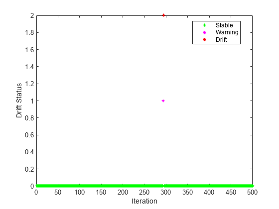
Plot the drift status.
gscatter(1:numIterations,dstatus,statusname,'gmr','*',4,'on',"Iteration","Drift Status")
xlim([0 numIterations])
Plot the performance metrics to see how they evolved during incremental learning.
figure
h = plot(mae.Variables);
xlim([0 numIterations])
ylim([0 4])
ylabel("Mean Absolute Deviation")
xlabel("Iteration")

xline(idaMdl.MetricsWarmupPeriod/numObsPerChunk,"g-.","Warmup Period",LineWidth= 1.5)
xline(idaMdl.TrainingPeriod/numObsPerChunk,"b-.","Training Period",LabelVerticalAlignment="middle",LineWidth= 1.5)
xline(driftTimes,"m--","Drift",LabelVerticalAlignment="middle",LineWidth=1.5)
legend(h,mae.Properties.VariableNames)
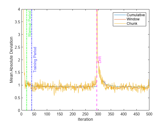
The plot suggests the following:
updateMetricscomputes the performance metrics after the metrics warm-up period only.updateMetricscomputes the cumulative metrics during each iteration.updateMetricscomputes the window metrics after processing 400 observationsBecause
idaMdlwas configured to predict observations from the beginning of incremental learning,losscan compute the MAD on each incoming chunk of data.
Plot the per observation loss.
figure()
plot(PoL,'b.');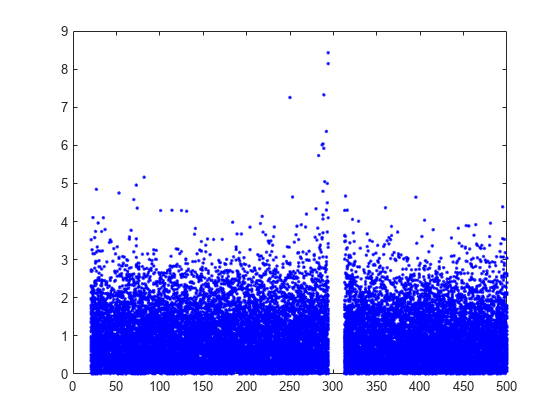
perObservationLoss computes the classification loss for each observation in the incoming chunk of data after the metrics warm-up period.
Input Arguments
Name-Value Arguments
References
Version History
Introduced in R2022b
See Also
predict | perObservationLoss | fit | incrementalDriftAwareLearner | updateMetrics | updateMetricsAndFit