predict

Predict response of nonlinear regression model

Syntax

ypred = predict(mdl,Xnew)

[ypred,yci] = predict(mdl,Xnew)

[ypred,yci] = predict(mdl,Xnew,Name,Value)

Description

ypred = predict(mdl,Xnew) returns the predicted response of the nonlinear regression model mdl to the points in Xnew.

[ypred,yci] = predict(mdl,Xnew) also returns confidence intervals for the responses at Xnew.

[ypred,yci] = predict(mdl,Xnew,Name,Value) specifies additional options using one or more name-value arguments. For example, you can specify the confidence level of the confidence interval and the prediction type.

Examples

Predict Responses

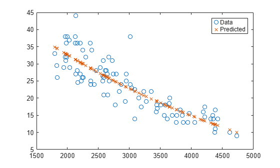
Create a nonlinear model of car mileage as a function of weight, and predict the response.

Create an exponential model of car mileage as a function of weight from the carsmall data. Scale the weight by a factor of 1000 so all the variables are roughly equal in size.

load carsmall
X = Weight;
y = MPG;
modelfun = 'y ~ b1 + b2*exp(-b3*x/1000)';
beta0 = [1 1 1];
mdl = fitnlm(X,y,modelfun,beta0);

Create predicted responses to the data.

Xnew = X;
ypred = predict(mdl,Xnew);

Plot the original responses and the predicted responses to see how they differ.

plot(X,y,'o',X,ypred,'x')
legend('Data','Predicted')

Confidence Intervals for Predictions

Create a nonlinear model of car mileage as a function of weight, and examine confidence intervals of some responses.

Create an exponential model of car mileage as a function of weight from the carsmall data. Scale the weight by a factor of 1000 so all the variables are roughly equal in size.

load carsmall
X = Weight;
y = MPG;
modelfun = 'y ~ b1 + b2*exp(-b3*x/1000)';
beta0 = [1 1 1];
mdl = fitnlm(X,y,modelfun,beta0);

Create predicted responses to the smallest, mean, and largest data points.

Xnew = [min(X);mean(X);max(X)];
[ypred,yci] = predict(mdl,Xnew)

ypred = 3×1

   34.9469
   22.6868
   10.0617

yci = 3×2

   32.5212   37.3726
   21.4061   23.9674
    7.0148   13.1086

Simultaneous Confidence Intervals for Robust Fit Curve

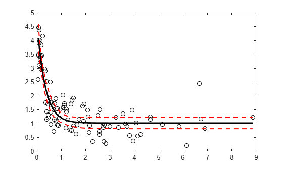
Generate sample data from the nonlinear regression model

$$y=b_1+b_2\exp (-b_{3}x)+ϵ$$

where $$b_1$$, $$b_2$$, and $$b_3$$ are coefficients, and the error term $$ϵ$$ is normally distributed with mean 0 and standard deviation 0.5.

modelfun = @(b,x)(b(1)+b(2)*exp(-b(3)*x));

rng('default') % For reproducibility
b = [1;3;2];
x = exprnd(2,100,1);
y = modelfun(b,x) + normrnd(0,0.5,100,1);

Fit the nonlinear model using robust fitting options.

opts = statset('nlinfit');
opts.RobustWgtFun = 'bisquare';
b0 = [2;2;2];
mdl = fitnlm(x,y,modelfun,b0,'Options',opts);

Plot the fitted regression model and simultaneous 95% confidence bounds.

xrange = [min(x):.01:max(x)]';
[ypred,yci] = predict(mdl,xrange,'Simultaneous',true);

figure()
plot(x,y,'ko') % observed data
hold on
plot(xrange,ypred,'k','LineWidth',2)
plot(xrange,yci','r--','LineWidth',1.5)

Confidence Interval Using Observation Weights

Load sample data.

S = load('reaction');
X = S.reactants;
y = S.rate;
beta0 = S.beta;

Specify a function handle for observation weights, then fit the Hougen-Watson model to the rate data using the specified observation weights function.

a = 1; b = 1;
weights = @(yhat) 1./((a + b*abs(yhat)).^2);
mdl = fitnlm(X,y,@hougen,beta0,'Weights',weights);

Compute the 95% prediction interval for a new observation with reactant levels [100,100,100] using the observation weight function.

[ypred,yci] = predict(mdl,[100,100,100],'Prediction','observation', ...
    'Weights',weights)

ypred = 
1.8149

yci = 1×2

    1.5264    2.1033

Input Arguments

mdl — Nonlinear regression model

NonLinearModel object

Nonlinear regression model, specified as a NonLinearModel object created using fitnlm.

Xnew — New predictor input values

table | matrix

New predictor input values, specified as a table or matrix. Each row of Xnew corresponds to one observation, and each column corresponds to one variable.

• If Xnew is a table, it must contain predictors that have the same names as predictors in the PredictorNames property of mdl.

• If Xnew is a matrix, it must have the same number of variables (columns) in the same order as the predictor input used to create mdl. All variables used to create mdl must be numeric. To treat numerical predictors as categorical, specify the predictors using the CategoricalVars name-value argument when you create mdl.

Note that Xnew must also contain any predictor variables not used as predictors in the fitted model.

Data Types: single | double | table

Name-Value Arguments

Specify optional pairs of arguments as Name1=Value1,...,NameN=ValueN, where Name is the argument name and Value is the corresponding value. Name-value arguments must appear after other arguments, but the order of the pairs does not matter.

Before R2021a, use commas to separate each name and value, and enclose Name in quotes.

Example: [ypred,yci] = predict(Mdl,Xnew,'Alpha',0.01,'Simultaneous',true) returns the confidence interval yci with a 99% confidence level, computed simultaneously for all predictor values.

Alpha — Significance level

0.05 (default) | numeric value in the range [0,1]

Significance level for the confidence interval, specified as a numeric value in the range [0,1]. The confidence level of yci is equal to 100(1 – Alpha)%. Alpha is the probability that the confidence interval does not contain the true value.

Example: Alpha=0.01

Data Types: single | double

Prediction — Prediction type

"curve" (default) | "observation"

Prediction type, specified as "curve" or "observation".

A regression model for the predictor variables X and the response variable y has the form

y = f(X) + ε,

where f is a fitted regression function and ε is a random noise term.

• If Prediction is "curve", then the function predicts confidence bounds for f(Xnew), the fitted responses at Xnew.

• If Prediction is "observation", then the function predicts confidence bounds for y, the response observations at Xnew.

The bounds for y are wider than the bounds for f(X) because of the additional variability of the noise term.

Example: Prediction="observation"

Data Types: string | char

Simultaneous — Flag to compute simultaneous confidence bounds

false or 0 (default) | true or 1

Flag to compute simultaneous confidence bounds, specified as a numeric or logical 1 (true) or 0 (false).

• true — predict calculates confidence bounds for the curve of response values corresponding to all predictor values in Xnew, using Schefféʼs method. The range between the upper and lower bounds contains the curve that consists of true response values with 100(1 – α)% confidence.

• false — predict calculates confidence bounds for the response value at each observation in Xnew. The confidence interval for a response value at a specific predictor value contains the true response value with 100(1 – α)% confidence.

With simultaneous bounds, the entire curve of true response values is within the bounds at high confidence. By contrast, nonsimultaneous bounds require only the response value at a single predictor value to be within the bounds at high confidence. Therefore, simultaneous bounds are wider than nonsimultaneous bounds.

Example: Simultaneous=true

W — Weights

no weights (default) | vector | function handle

Vector of real, positive value weights or a function handle.

• If you specify a vector, then it must have the same number of elements as the number of observations (or rows) in Xnew.

• If you specify a function handle, the function must accept a vector of predicted response values as input, and returns a vector of real positive weights as output.

Given weights, W, predict estimates the error variance at observation i by MSE*(1/W(i)), where MSE is the mean squared error.

Output Arguments

ypred — Predicted response values

numeric vector

Predicted response values evaluated at Xnew, returned as a numeric vector.

yci — Confidence intervals for responses

two-column numeric matrix

Confidence intervals for the responses, returned as a two-column matrix in which each row provides one interval. The meaning of the confidence interval depends on the settings of the name-value arguments Alpha, Prediction, and Simultaneous.

Tips

• For predictions with added noise, use random.

• For a syntax that can be easier to use with models created from tables or dataset arrays, try feval.

References

[1] Lane, T. P. and W. H. DuMouchel. “Simultaneous Confidence Intervals in Multiple Regression.” The American Statistician. Vol. 48, No. 4, 1994, pp. 315–321. Available at https://doi.org/10.1080/00031305.1994.10476090

[2] Seber, G. A. F., and C. J. Wild. Nonlinear Regression. Hoboken, NJ: Wiley-Interscience, 2003.

Version History

Introduced in R2012a