profileLikelihood
Syntax
Description
[___] = profileLikelihood(
specifies additional options using one or more name-value arguments. For example, you can
specify the significance level for the confidence interval and the values for the
coefficient of interest. mdl,coef,Name=Value)
Examples
Load a table of standardized variables generated from the carbig data set.
load standardizedcar.matThe table tbl contains the variables Horsepower, Weight, and MPG, which represent car horsepower, weight, and miles per gallon, respectively.
Fit a nonlinear model to the data using Horsepower and Weight as predictors, and MPG as the response.
modelfun = @(b,x) exp(b(1)*x(:,1))+b(2)*x(:,2)+b(3);
beta0 = [1 1 1];
mdl = fitnlm(tbl,modelfun,beta0)
mdl =
Nonlinear regression model:
    MPG ~ exp(b1*Horsepower) + b2*Weight + b3

Estimated Coefficients:
          Estimate       SE        tStat       pValue
          ________    ________    _______    ___________

    b1    -0.57016    0.045819    -12.444     3.7325e-30
    b2    -0.39274    0.043737    -8.9797     1.1804e-17
    b3     -1.1417    0.034104    -33.476    1.3291e-116


Number of observations: 392, Error degrees of freedom: 389
Root Mean Squared Error: 0.516
R-Squared: 0.735,  Adjusted R-Squared 0.733
F-statistic vs. constant model: 539, p-value = 8.27e-113
mdl contains a fitted nonlinear regression model. The coefficient b1 is a nonlinear coefficient because it is inside the exponential term in the model function.
Calculate the profile loglikelihood and confidence interval for b1.
[LV,PV,CI] = profileLikelihood(mdl,"b1");
CI
CI = 1×2
-0.6597 -0.4660
The output shows the 95% likelihood-ratio confidence interval for b1.
Plot the profile loglikelihood values for b1 using the plotProfileLikelihood function.
plotProfileLikelihood(mdl,"b1")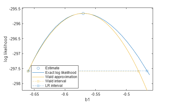
The plot shows the loglikelihood values together with the estimated value for b1, the Wald approximation, and the Wald and likelihood-ratio confidence intervals. The calculated values for b1 cover the confidence intervals, and the maximum likelihood estimate for b1 appears at the peak of the profile loglikelihood, confirming it is the maximum likelihood estimate. The likelihood-ratio confidence interval is slightly wider than the Wald interval, and is also asymmetric. However, the closeness of the two intervals suggests that the assumptions of the Wald approximation hold true for this model.
Load the reaction data set.
load reactionThe variables reactants and rate contain data for the partial pressures of three chemicals and their reactant rates. The vector beta contains initial values for the Hougen-Watson model coefficients.
Fit the Hougen-Watson model to the data using the hougen function. Use reactants as the predictor data and rate as the response.
mdl = fitnlm(reactants,rate,@hougen,beta)
mdl =
Nonlinear regression model:
    y ~ hougen(b,X)

Estimated Coefficients:
          Estimate       SE       tStat     pValue
          ________    ________    ______    _______

    b1      1.2526     0.86701    1.4447    0.18654
    b2    0.062776    0.043561    1.4411    0.18753
    b3    0.040048    0.030885    1.2967    0.23089
    b4     0.11242    0.075157    1.4957    0.17309
    b5      1.1914     0.83671    1.4239     0.1923


Number of observations: 13, Error degrees of freedom: 8
Root Mean Squared Error: 0.193
R-Squared: 0.999,  Adjusted R-Squared 0.998
F-statistic vs. zero model: 3.91e+03, p-value = 2.54e-13
mdl contains the fitted nonlinear regression model. The estimate for b2 is near 0.06 and has a large p-value.
Calculate the profile loglikelihood for b2 in an interval around its estimated value. Plot the loglikelihood values against the specified values for b2.
[LV2,PV2] = profileLikelihood(mdl,"b2",CoefficientValues=[0.01:0.01:1]);
plot(PV2,LV2)
xlabel("b2")
ylabel("loglikelihood")
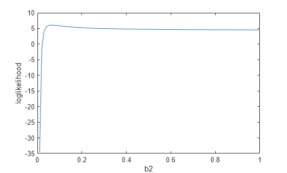
The profile loglikelihood has a nonlinear elbow shape and does not change significantly for values of b2 larger than 0.1. This result is consistent with the large p-value, which suggests that b2 does not have a statistically significant effect on the response variable.
Input Arguments
Name-Value Arguments
Output Arguments
More About
Alternative Functionality
You can calculate both Wald and likelihood-ratio confidence intervals for several
coefficients using the coefCI function.
Version History
Introduced in R2025a