pdist2

R2026b

Pairwise distance between two sets of observations

Syntax

D = pdist2(X,Y,Distance)

D = pdist2(X,Y,Distance,DistParameter)

D = pdist2(___,Name,Value)

[D,I] = pdist2(___)

Description

D = pdist2(X,Y,Distance) returns the distance between each pair of observations in X and Y using the metric specified by Distance.

D = pdist2(X,Y,Distance,DistParameter) returns the distance using the metric specified by Distance and DistParameter. You can specify DistParameter only when Distance is "seuclidean", "minkowski", or "mahalanobis".

D = pdist2(___,Name,Value), for any previous arguments, modifies the computation using name-value parameters. For example,

• D = pdist2(X,Y,Distance,'Smallest',K) computes the distance using the metric specified by Distance and returns the K smallest pairwise distances to observations in X for each observation in Y in ascending order.

• D = pdist2(X,Y,Distance,DistParameter,'Largest',K) computes the distance using the metric specified by Distance and DistParameter and returns the K largest pairwise distances in descending order.

[D,I] = pdist2(___) also returns the matrix I. The matrix I contains the indices of the observations in X corresponding to the distances in D. You must specify Smallest or Largest to return I.

Examples

Compute Euclidean Distance

Create two matrices with three observations and two variables.

rng('default') % For reproducibility
X = rand(3,2);
Y = rand(3,2);

Compute the Euclidean distance. The default value of the input argument Distance is 'euclidean'. When computing the Euclidean distance without using a name-value pair argument, you do not need to specify Distance.

D = pdist2(X,Y)

D = 3×3

    0.5387    0.8018    0.1538
    0.7100    0.5951    0.3422
    0.8805    0.4242    1.2050

D(i,j) corresponds to the pairwise distance between observation i in X and observation j in Y.

Compute Minkowski Distance

Create two matrices with three observations and two variables.

rng('default') % For reproducibility
X = rand(3,2);
Y = rand(3,2);

Compute the Minkowski distance with the default exponent 2.

D1 = pdist2(X,Y,'minkowski')

D1 = 3×3

    0.5387    0.8018    0.1538
    0.7100    0.5951    0.3422
    0.8805    0.4242    1.2050

Compute the Minkowski distance with an exponent of 1, which is equal to the city block distance.

D2 = pdist2(X,Y,'minkowski',1)

D2 = 3×3

    0.5877    1.0236    0.2000
    0.9598    0.8337    0.3899
    1.0189    0.4800    1.7036

D3 = pdist2(X,Y,'cityblock')

D3 = 3×3

    0.5877    1.0236    0.2000
    0.9598    0.8337    0.3899
    1.0189    0.4800    1.7036

Compute Mahalanobis Distance

Create two matrices with five observations and two variables.

rng(0,"twister") % For reproducibility
X = rand(5,2);
Y = rand(5,2);

Compute the Mahalanobis distance using the pdist2 function.

D = pdist2(X,Y,"mahalanobis")

D = 5×5

    2.0012    0.9926    2.1767    1.9656    2.2036
    2.3429    0.4318    1.6528    1.7564    1.7453
    1.0330    2.5697    2.7833    1.3093    2.3936
    3.2463    1.3676    0.1638    1.4094    0.3452
    2.6608    1.6585    0.9895    0.6572    0.5121

Compute the Mahalanobis distance between the mean of X and the observations Y. Use the covariance of X for the distance metric parameter.

D2 = pdist2(mean(X),Y,"mahalanobis",cov(X))

D2 = 1×5

    2.0090    0.9377    1.2824    0.7850    1.0966

Compute the squared Mahalanobis distance using the mahal function.

SqMahalDist = mahal(Y,X)'

SqMahalDist = 1×5

    4.0360    0.8792    1.6445    0.6162    1.2025

Compute the square root of each value.

MahalDist = SqMahalDist.^0.5

MahalDist = 1×5

    2.0090    0.9377    1.2824    0.7850    1.0966

The Mahalanobis distance values are the same as those returned by the pdist2 function.

Find the Two Smallest Pairwise Distances

Create two matrices with three observations and two variables.

rng('default') % For reproducibility
X = rand(3,2);
Y = rand(3,2);

Find the two smallest pairwise Euclidean distances to observations in X for each observation in Y.

[D,I] = pdist2(X,Y,'euclidean','Smallest',2)

D = 2×3

    0.5387    0.4242    0.1538
    0.7100    0.5951    0.3422

I = 2×3

     1     3     1
     2     2     2

For each observation in Y, pdist2 finds the two smallest distances by computing and comparing the distance values to all the observations in X. The function then sorts the distances in each column of D in ascending order. I contains the indices of the observations in X corresponding to the distances in D.

Compute Pairwise Distance Between Tables of Mixed Data

Since R2026b

Compute the distance between two tables containing both continuous and categorical data.

Create two tables with five observations and three variables each. The first two variables contain continuous data in the interval (0,1), and the third variable contains integers between 1 and 3.

rng("default") % For reproducibility
X = table(rand(5,1),rand(5,1),randi(3,5,1))

X = 5×3 table
     Var1       Var2      Var3
    _______    _______    ____

    0.81472    0.09754     1  
    0.90579     0.2785     3  
    0.12699    0.54688     3  
    0.91338    0.95751     2  
    0.63236    0.96489     3  

Y = table(rand(5,1),rand(5,1),randi(3,5,1))

Y = 5×3 table
     Var1        Var2      Var3
    _______    ________    ____

    0.14189     0.65574     3  
    0.42176    0.035712     3  
    0.91574     0.84913     2  
    0.79221     0.93399     2  
    0.95949     0.67874     1  

Compute the modified Goodall distance. Treat the third variable as categorical.

D = pdist2(X,Y,"goodall3",CategoricalVariables="Var3")

D = 5×5

    0.6000    0.5000    0.6333    0.5333    0.3222
    0.4000    0.4333    0.5000    0.5333    0.5000
    0.2000    0.3667    0.6333    0.4667    0.6333
    0.6000    0.8333    0.0556    0.2222    0.3667
    0.2667    0.5000    0.6333    0.4667    0.6333

Accelerate Distance Computation Using fasteuclidean Distance

Create two large matrices of points, and then measure the time used by pdist2 with the default "euclidean" distance metric.

rng default % For reproducibility
N = 10000;
X = randn(N,1000);
Y = randn(N,1000);
D = pdist2(X,Y); % Warm up function for more reliable timing information
tic
D = pdist2(X,Y);
standard = toc

standard = 
6.3820

Next, measure the time used by pdist2 with the "fasteuclidean" distance metric. Specify a cache size of 100.

D = pdist2(X,Y,"fasteuclidean",CacheSize=100); % Warm up function
tic
D2 = pdist2(X,Y,"fasteuclidean",CacheSize=100);
accelerated = toc

accelerated = 
1.2317

Evaluate how many times faster the accelerated computation is compared to the standard.

standard/accelerated

ans = 
5.1816

The accelerated version is more than twice as fast for this example.

Compute Pairwise Distance with Missing Elements Using a Custom Distance Function

Define a custom distance function that ignores coordinates with NaN values, and compute pairwise distance by using the custom distance function.

Create two matrices with three observations and three variables.

rng('default') % For reproducibility
X = rand(3,3)
Y = [X(:,1:2) rand(3,1)]

X =

    0.8147    0.9134    0.2785
    0.9058    0.6324    0.5469
    0.1270    0.0975    0.9575


Y =

    0.8147    0.9134    0.9649
    0.9058    0.6324    0.1576
    0.1270    0.0975    0.9706

The first two columns of X and Y are identical. Assume that X(1,1) is missing.

X(1,1) = NaN

X =

       NaN    0.9134    0.2785
    0.9058    0.6324    0.5469
    0.1270    0.0975    0.9575

Compute the Hamming distance.

D1 = pdist2(X,Y,'hamming')

D1 =

       NaN       NaN       NaN
    1.0000    0.3333    1.0000
    1.0000    1.0000    0.3333

If observation i in X or observation j in Y contains NaN values, the function pdist2 returns NaN for the pairwise distance between i and j. Therefore, D1(1,1), D1(1,2), and D1(1,3) are NaN values.

Define a custom distance function nanhamdist that ignores coordinates with NaN values and computes the Hamming distance. When working with a large number of observations, you can compute the distance more quickly by looping over coordinates of the data.

function D2 = nanhamdist(XI,XJ)  
%NANHAMDIST Hamming distance ignoring coordinates with NaNs
[m,p] = size(XJ);
nesum = zeros(m,1);
pstar = zeros(m,1);
for q = 1:p
    notnan = ~(isnan(XI(q)) | isnan(XJ(:,q)));
    nesum = nesum + ((XI(q) ~= XJ(:,q)) & notnan);
    pstar = pstar + notnan;
end
D2 = nesum./pstar; 

Compute the distance with nanhamdist by passing the function handle as an input argument of pdist2.

D2 = pdist2(X,Y,@nanhamdist)

D2 =

    0.5000    1.0000    1.0000
    1.0000    0.3333    1.0000
    1.0000    1.0000    0.3333

Assign New Data to Existing Clusters and Generate C/C++ Code

kmeans performs k-means clustering to partition data into k clusters. When you have a new data set to cluster, you can create new clusters that include the existing data and the new data by using kmeans. The kmeans function supports C/C++ code generation, so you can generate code that accepts training data and returns clustering results, and then deploy the code to a device. In this workflow, you must pass training data, which can be of considerable size. To save memory on the device, you can separate training and prediction by using kmeans and pdist2, respectively.

Use kmeans to create clusters in MATLAB® and use pdist2 in the generated code to assign new data to existing clusters. For code generation, define an entry-point function that accepts the cluster centroid positions and the new data set, and returns the index of the nearest cluster. Then, generate code for the entry-point function.

Generating C/C++ code requires MATLAB® Coder™.

Perform k-Means Clustering

Generate a training data set using three distributions.

rng('default') % For reproducibility
X = [randn(100,2)*0.75+ones(100,2);
    randn(100,2)*0.5-ones(100,2);
    randn(100,2)*0.75];

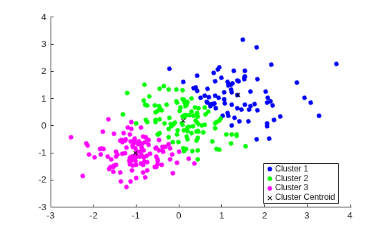
Partition the training data into three clusters by using kmeans.

[idx,C] = kmeans(X,3);

Plot the clusters and the cluster centroids.

figure
gscatter(X(:,1),X(:,2),idx,'bgm')
hold on
plot(C(:,1),C(:,2),'kx')
legend('Cluster 1','Cluster 2','Cluster 3','Cluster Centroid')

Assign New Data to Existing Clusters

Generate a test data set.

Xtest = [randn(10,2)*0.75+ones(10,2);
    randn(10,2)*0.5-ones(10,2);
    randn(10,2)*0.75];

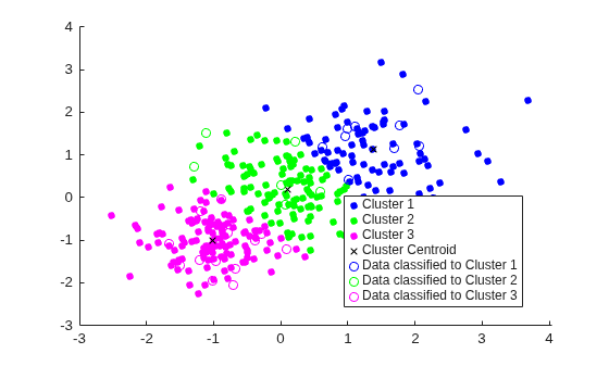
Classify the test data set using the existing clusters. Find the nearest centroid from each test data point by using pdist2.

[~,idx_test] = pdist2(C,Xtest,'euclidean','Smallest',1);

Plot the test data and label the test data using idx_test by using gscatter.

gscatter(Xtest(:,1),Xtest(:,2),idx_test,'bgm','ooo')
legend('Cluster 1','Cluster 2','Cluster 3','Cluster Centroid', ...
    'Data classified to Cluster 1','Data classified to Cluster 2', ...
    'Data classified to Cluster 3')

Generate Code

Generate C code that assigns new data to the existing clusters. Note that generating C/C++ code requires MATLAB® Coder™.

Define an entry-point function named findNearestCentroid that accepts centroid positions and new data, and then find the nearest cluster by using pdist2.

Add the %#codegen compiler directive (or pragma) to the entry-point function after the function signature to indicate that you intend to generate code for the MATLAB algorithm. Adding this directive instructs the MATLAB Code Analyzer to help you diagnose and fix violations that would cause errors during code generation.

type findNearestCentroid % Display contents of findNearestCentroid.m

function idx = findNearestCentroid(C,X) %#codegen
[~,idx] = pdist2(C,X,'euclidean','Smallest',1); % Find the nearest centroid

Note: If you click the button located in the upper-right section of this page and open this example in MATLAB®, then MATLAB® opens the example folder. This folder includes the entry-point function file.

Generate code by using codegen (MATLAB Coder). Because C and C++ are statically typed languages, you must determine the properties of all variables in the entry-point function at compile time. To specify the data type and array size of the inputs of findNearestCentroid, pass a MATLAB expression that represents the set of values with a certain data type and array size by using the -args option. For details, see Specify Variable-Size Arguments for Code Generation of Machine Learning Models.

codegen findNearestCentroid -args {C,Xtest}

Code generation successful.

codegen generates the MEX function findNearestCentroid_mex with a platform-dependent extension.

Verify the generated code.

myIndx = findNearestCentroid(C,Xtest);
myIndex_mex = findNearestCentroid_mex(C,Xtest);
verifyMEX = isequal(idx_test,myIndx,myIndex_mex)

verifyMEX = logical
   1

isequal returns logical 1 (true), which means all the inputs are equal. The comparison confirms that the pdist2 function, the findNearestCentroid function, and the MEX function return the same index.

You can also generate optimized CUDA® code using GPU Coder™.

cfg = coder.gpuConfig('mex');
codegen -config cfg findNearestCentroid -args {C,Xtest}

For more information on code generation, see Introduction to Code Generation for Statistics and Machine Learning Functions. For more information on GPU coder, see Get Started with GPU Coder (GPU Coder) and Functions and Objects Supported for GPU Code Generation (GPU Coder).

Input Arguments

X,Y — Input data

numeric matrix | table

Input data, specified as a numeric matrix or table. X is an mx-by-n matrix or table, and Y is an my-by-n matrix or table. Rows correspond to individual observations, and columns correspond to individual variables.

If X and Y are tables, they must have the same variable names.

Data Types: single | double | table

Distance — Distance metric

character vector | string scalar | function handle

Distance metric, specified as a character vector, string scalar, or function handle.

• If all the variables are continuous, then you can specify one of these distance metrics.

  Value	Description
  "euclidean"	Euclidean distance
  "squaredeuclidean"	Squared Euclidean distance. (This option is provided for efficiency only. It does not satisfy the triangle inequality.)
  "seuclidean"	Standardized Euclidean distance. Each coordinate difference between observations is scaled by dividing by the corresponding element of the standard deviation, S = std(X,"omitnan"). Use DistParameter to specify a different value for S.
  "fasteuclidean"	Euclidean distance computed by using an alternative algorithm that saves time when the number of predictors is at least 10. In some cases, this faster algorithm can reduce accuracy. Algorithms starting with "fast" do not support sparse data. For details, see Algorithms.
  "fastsquaredeuclidean"	Squared Euclidean distance computed by using an alternative algorithm that saves time when the number of predictors is at least 10. In some cases, this faster algorithm can reduce accuracy. Algorithms starting with "fast" do not support sparse data. For details, see Algorithms.
  "fastseuclidean"	Standardized Euclidean distance computed by using an alternative algorithm that saves time when the number of predictors is at least 10. In some cases, this faster algorithm can reduce accuracy. Algorithms starting with "fast" do not support sparse data. For details, see Algorithms.
  "mahalanobis"	Mahalanobis distance, computed using the sample covariance of X, C = cov(X,"omitrows"). Use DistParameter to specify a different value for C, where the matrix C is symmetric and positive definite.
  "cityblock"	City block distance
  "minkowski"	Minkowski distance. The default exponent is 2. Use DistParameter to specify a different exponent P, where P is a positive scalar value of the exponent.
  "chebychev"	Chebychev distance (maximum coordinate difference)
  "cosine"	One minus the cosine of the included angle between points (treated as vectors)
  "correlation"	One minus the sample correlation between points (treated as sequences of values)
  "jaccard"	One minus the Jaccard coefficient, which is the percentage of nonzero coordinates that differ
  "spearman"	One minus the sample Spearman's rank correlation between observations (treated as sequences of values)

• If all the variables are categorical, then you can specify the following distance metric.

  Value	Description
  "hamming"	Hamming distance, which is the percentage of coordinates that differ

• If all the variables are a mix of continuous and categorical variables, then you can specify the following distance metric.

  Value	Description
  "goodall3" (since R2026b)	Modified Goodall distance

• To specify a custom distance metric, use function handle notation. A distance function has the form

  function D2 = distfun(ZI,ZJ)
  % calculation of distance
  ...

  where

  • ZI is a 1-by-n vector containing a single observation.

  • ZJ is an m2-by-n matrix containing multiple observations. distfun must accept a matrix ZJ with an arbitrary number of observations.

  • D2 is an m2-by-1 vector of distances, and D2(k) is the distance between observations ZI and ZJ(k,:).

  If your data is not sparse, you can generally compute distances more quickly by using a built-in distance metric instead of a function handle.

The default value of Distance is "euclidean" if all the variables are continuous, "hamming" if all the variables are categorical, and "goodall3" if the variables are a mix of continuous and categorical. For more information on the distance metrics, see Distance Metrics.

When you use "seuclidean", "minkowski", or "mahalanobis", you can specify an additional input argument DistParameter to control these metrics. You can also use these metrics in the same way as the other metrics with the default value of DistParameter.

Example: "minkowski"

Data Types: char | string | function_handle

DistParameter — Distance metric parameter values

positive scalar | numeric vector | numeric matrix

Distance metric parameter values, specified as a positive scalar, numeric vector, or numeric matrix. You can specify this argument only when Distance is "seuclidean", "fastseuclidean", "minkowski", or "mahalanobis".

• If Distance is "seuclidean" or "fastseuclidean", then DistParameter must be a vector of nonnegative values with length equal to the number of columns in X. The default value is std(X,"omitnan").

• If Distance is "minkowski", DistParameter is the exponent of the Minkowski distance, specified as a positive scalar. The default value is 2.

• If Distance is "mahalanobis", DistParameter is a covariance matrix, specified as a square numeric matrix with the same number of columns as X. The default value is cov(X,"omitrows"). DistParameter must be symmetric and positive definite.

Example: 3

Data Types: single | double

Name-Value Arguments

Specify optional pairs of arguments as Name1=Value1,...,NameN=ValueN, where Name is the argument name and Value is the corresponding value. Name-value arguments must appear after other arguments, but the order of the pairs does not matter.

Before R2021a, use commas to separate each name and value, and enclose Name in quotes.

Example: Either Smallest = K or Largest = K. You cannot use both Smallest and Largest.

CacheSize — Size of Gram matrix in megabytes

1e3 (default) | positive scalar | 'maximal'

Size of the Gram matrix in megabytes, specified as a positive scalar or 'maximal'. The pdist2 function can use CacheSize only when the Distance argument begins with fast.

If 'maximal', pdist2 attempts to allocate enough memory for an entire intermediate matrix whose size is MX-by-MY, where MX is the number of rows of the input data X, and MY is the number of rows of the input data Y. The cache size does not have to be large enough for an entire intermediate matrix, but must be at least large enough to hold an MX-by-1 vector. Otherwise, pdist2 uses the regular algorithm for computing Euclidean distance.

If the distance argument begins with fast and CacheSize is too large or is 'maximal', pdist2 can attempt to allocate a Gram matrix that exceeds the available memory. In this case, MATLAB^® issues an error.

Example: CacheSize='maximal'

Data Types: double | char | string

Smallest — Number of smallest distances to find

positive integer

Number of smallest distances to find, specified as the comma-separated pair consisting of 'Smallest' and a positive integer. If you specify 'Smallest', then pdist2 sorts the distances in each column of D in ascending order. You can use only one of the arguments Smallest and Largest.

Example: 'Smallest',3

Data Types: single | double

Largest — Number of largest distances to find

positive integer

Number of largest distances to find, specified as the comma-separated pair consisting of 'Largest' and a positive integer. If you specify 'Largest', then pdist2 sorts the distances in each column of D in descending order. You can use only one of the arguments Smallest and Largest.

Example: 'Largest',3

Data Types: single | double

VariableNames — Variables to include in computation

string array (default) | character vector | cell array of character vectors

Since R2026b

Variables to include in the computation, specified as a string array, character vector, or cell array of character vectors. Because matrices do not have named variables, this argument applies only when the input data consists of tables.

By default, VariableNames contains all the variables in X and Y.

Example: VariableNames=["Name","Age","Score"]

Data Types: char | string | cell

CategoricalVariables — Variables to treat as categorical

"all" | vector of numeric indices | logical vector | string scalar | character vector | string array | cell array of character vectors

Since R2026b

Variables to treat as categorical, specified as one of the values in this table.

Value	Description
"all"	All variables contain categorical values.
Vector of numeric indices	Each vector element corresponds to the index of a variable, indicating that the variable contains categorical values.
Logical vector	A logical vector the same length as VariableNames. A value of true indicates that the corresponding variable contains categorical values.
Character vector or string scalar (for one variable) String array or cell array of character vectors (for multiple variables)	An array containing the names of variables with categorical values. The array elements must be names found in VariableNames.

If X and Y are numeric matrices, CategoricalVariables cannot be a string array, cell array of character vectors, character vector, or string scalar. By default, pdist2 assumes that all variables in numeric matrices are continuous.

If X and Y are tables, the function assumes that a variable is categorical if it is a logical vector, an unordered categorical vector, a string array, or a cell array of character vectors.

Example: CategoricalVariables="all"

Data Types: single | double | logical | char | string | cell

Output Arguments

D — Pairwise distances

numeric matrix

Pairwise distances, returned as a numeric matrix.

If you do not specify either 'Smallest' or 'Largest', then D is an mx-by-my matrix, where mx and my are the number of observations in X and Y, respectively. D(i,j) is the distance between observation i in X and observation j in Y. If observation i in X or observation j in Y contains NaN, then D(i,j) is NaN for the built-in distance functions.

If you specify either 'Smallest' or 'Largest' as K, then D is a K-by-my matrix. D contains either the K smallest or K largest pairwise distances to observations in X for each observation in Y. For each observation in Y, pdist2 finds the K smallest or largest distances by computing and comparing the distance values to all the observations in X. If K is greater than mx, pdist2 returns an mx-by-my matrix.

I — Sort index

positive integer matrix

Sort index, returned as a positive integer matrix. I is the same size as D. I contains the indices of the observations in X corresponding to the distances in D. You must specify Smallest or Largest to return I.

More About

Distance Metrics

A distance metric is a function that defines the distance between two observations. pdist2 supports the following distance metrics: Euclidean, standardized Euclidean, Mahalanobis, city block, Minkowski, Chebychev, cosine, correlation, Hamming, Jaccard, Spearman, and modified Goodall. Specify the distance metric using the Distance name-value argument.

Given an mx-by-n data matrix or table X, which is treated as mx (1-by-n) row vectors x₁, x₂, ..., x_mx, and an my-by-n data matrix or table Y, which is treated as my (1-by-n) row vectors y₁, y₂, ...,y_my, the various distances between the vector x_s and y_t are defined as follows:

• Euclidean distance

  $$d_{st}^2=(x_s-y_t)(x_s-y_t{)}^{\prime }.$$

  The Euclidean distance is a special case of the Minkowski distance, where p = 2.

• Standardized Euclidean distance

  $$d_{st}^2=(x_s-y_t)V^{-1}(x_s-y_t{)}^{\prime },$$

  where V is the n-by-n diagonal matrix whose jth diagonal element is (S(j))², where S is a vector of scaling factors for each dimension.

• Fast Euclidean distance is the same as Euclidean distance, computed by using an alternative algorithm that saves time when the number of predictors is at least 10. In some cases, this faster algorithm can reduce accuracy. Does not support sparse data. See Fast Euclidean Distance Algorithm.

• Fast standardized Euclidean distance is the same as standardized Euclidean distance, computed by using an alternative algorithm that saves time when the number of predictors is at least 10. In some cases, this faster algorithm can reduce accuracy. Does not support sparse data. See Fast Euclidean Distance Algorithm.

• Mahalanobis distance

  $$d_{st}^2=(x_s-y_t)C^{-1}(x_s-y_t{)}^{\prime },$$

  where C is the covariance matrix.

• City block distance

  $$d_{st}={\displaystyle \sum _{j=1}^n\left|x_{sj}-y_{tj}\right|}.$$

  The city block distance is a special case of the Minkowski distance, where p = 1.

• Minkowski distance

  $$d_{st}=\sqrt[p]{{\displaystyle \sum _{j=1}^n{\left|x_{sj}-y_{tj}\right|}^p}}.$$

  For the special case of p = 1, the Minkowski distance gives the city block distance. For the special case of p = 2, the Minkowski distance gives the Euclidean distance. For the special case of p = ∞, the Minkowski distance gives the Chebychev distance.

• Chebychev distance

  $$d_{st}={\max }_j\left\{\left|x_{sj}-y_{tj}\right|\right\}.$$

  The Chebychev distance is a special case of the Minkowski distance, where p = ∞.

• Cosine distance

  $$d_{st}=\left(1-\frac{x_s{y^{\prime }}_t}{\sqrt{\left(x_s{x^{\prime }}_s\right)\left(y_t{y^{\prime }}_t\right)}}\right).$$

• Correlation distance

  $$d_{st}=1-\frac{\left(x_s-{\overline{x}}_s\right){\left(y_t-{\overline{y}}_t\right)}^{\prime }}{\sqrt{\left(x_s-{\overline{x}}_s\right){\left(x_s-{\overline{x}}_s\right)}^{\prime }}\sqrt{\left(y_t-{\overline{y}}_t\right){\left(y_t-{\overline{y}}_t\right)}^{\prime }}},$$

  where

  $${\overline{x}}_s=\frac{1}{n}{\displaystyle \sum _j{x}_{sj}}$$

  and

  $${\overline{y}}_t=\frac{1}{n}{\displaystyle \sum _j{y}_{tj}}.$$

• Hamming distance

  $$d_{st}=(\#(x_{sj}\ne y_{tj})/n).$$

  The Hamming distance is the percentage of coordinates that differ.

• Jaccard distance is one minus the Jaccard coefficient, which is the percentage of nonzero coordinates that differ:

  $$d_{st}=\frac{\#\left[\left(x_{sj}\ne y_{tj}\right)\cap \left(\left(x_{sj}\ne 0\right)\cup \left(y_{tj}\ne 0\right)\right)\right]}{\#\left[\left(x_{sj}\ne 0\right)\cup \left(y_{tj}\ne 0\right)\right]}.$$

• Spearman distance is one minus the sample Spearman's rank correlation between observations (treated as sequences of values):

  $$d_{st}=1-\frac{\left(r_s-{\overline{r}}_s\right){\left(r_t-{\overline{r}}_t\right)}^{\prime }}{\sqrt{\left(r_s-{\overline{r}}_s\right){\left(r_s-{\overline{r}}_s\right)}^{\prime }}\sqrt{\left(r_t-{\overline{r}}_t\right){\left(r_t-{\overline{r}}_t\right)}^{\prime }}},$$

  where

  • r_sj is the rank of x_sj taken over x_s1, x_s2, ...x_s,n, as computed by tiedrank.

  • r_tj is the rank of y_tj taken over y_t1, y_t2, ...y_t,n, as computed by tiedrank.

  • r_s and r_t are the coordinate-wise rank vectors of x_s and y_t, that is, r_s = (r_s1, r_s2, ... r_sn) and r_t = (r_t1, r_t2, ... r_tn).

  • $${\overline{r}}_s=\frac{1}{n}{\displaystyle \sum _j{r}_{sj}}=\frac{\left(n+1\right)}{2}$$.

  • $${\overline{r}}_t=\frac{1}{n}{\displaystyle \sum _j{r}_{tj}}=\frac{\left(n+1\right)}{2}$$.

• Modified Goodall distance

  This distance is a variant of the Goodall distance, which assigns a small distance if the matching values are infrequent regardless of the frequencies of the other values. For mismatches, the distance contribution of the predictor is 1/(number of variables).

Algorithms

Fast Euclidean Distance Algorithm

The Distance argument values that begin with fast (such as "fasteuclidean" and "fastseuclidean") calculate Euclidean distances using an algorithm that uses extra memory to save computational time. This algorithm is named "Euclidean Distance Matrix Trick" in Albanie [1] and elsewhere. Internal testing shows that this algorithm saves time when the number of predictors is at least 10. Algorithms starting with fast do not support sparse data.

To find the matrix D of distances between all the points x_i and x_j, where each x_i has n variables, the algorithm computes distance using the final line in the following equations:

$$\begin{array}{c}{D}_{i,j}^2=\Vert x_i-x_j{\Vert }^2\\ ={(}^{x_i}(x_i-x_j)\\ =\Vert x_i{\Vert }^2-2x_i^T{x}_j+\Vert x_j{\Vert }^2.\end{array}$$

The matrix $$x_i^T{x}_j$$ in the last line of the equations is called the Gram matrix. Computing the set of squared distances is faster, but slightly less numerically stable, when you compute and use the Gram matrix instead of computing the squared distances by squaring and summing. For more details, see Albanie [1].

To store the Gram matrix, the software uses a cache with the default size of 1e3 megabytes. You can set the cache size using the CacheSize name-value argument. If the value of CacheSize is too large or "maximal", then the software might try to allocate a Gram matrix that exceeds the available memory. In this case, the software issues an error.

References

[1] Albanie, Samuel. Euclidean Distance Matrix Trick. June, 2019. Available at https://samuelalbanie.com/files/Euclidean_distance_trick.pdf.

Extended Capabilities

Tall Arrays

Calculate with arrays that have more rows than fit in memory.

The pdist2 function supports tall arrays with the following usage notes and limitations:

• The first input X must be a tall array. Input Y cannot be a tall array.

For more information, see Tall Arrays.

C/C++ Code Generation

Generate C and C++ code using MATLAB® Coder™.

Usage notes and limitations:

• The distance input argument value (Distance) must be a compile-time constant. For example, to use the Minkowski distance, include coder.Constant('Minkowski') in the -args value of codegen.

• The distance input argument value (Distance) cannot be a custom distance function.

• pdist2 does not support code generation for fast Euclidean distance computations, meaning those distance metrics whose names begin with fast (for example, 'fasteuclidean').

• Names in name-value arguments must be compile-time constants. For example, to use the 'Smallest' name-value pair argument in the generated code, include {coder.Constant('Smallest'),0} in the -args value of codegen (MATLAB Coder).

• The sorted order of tied distances in the generated code can be different from the order in MATLAB due to numerical precision.

• The generated code of pdist2 uses parfor (MATLAB Coder) to create loops that run in parallel on supported shared-memory multicore platforms in the generated code. If your compiler does not support the Open Multiprocessing (OpenMP) application interface or you disable OpenMP library, MATLAB Coder™ treats the parfor-loops as for-loops. To find supported compilers, see Supported Compilers. To disable OpenMP library, set the EnableOpenMP property of the configuration object to false. For details, see coder.CodeConfig (MATLAB Coder).

• pdist2 returns integer-type (int32) indices in generated standalone C/C++ code. Therefore, the function allows for strict single-precision support when you use single-precision inputs. For MEX code generation, the function still returns double-precision indices to match the MATLAB behavior.

For more information on code generation, see Introduction to Code Generation for Statistics and Machine Learning Functions and Overview of Code Generation Using MATLAB Coder (MATLAB Coder).

GPU Code Generation

Generate CUDA® code for NVIDIA® GPUs using GPU Coder™.

Usage notes and limitations:

• The supported distance input argument values (Distance) for optimized CUDA code are "euclidean", "squaredeuclidean", "seuclidean", "mahalanobis", "cityblock", "minkowski", "chebychev", "cosine", "correlation", "hamming", and "jaccard".

• Distance cannot be a custom distance function.

• Distance must be a compile-time constant.

• Names in name-value pair arguments must be compile-time constants.

• The sorted order of tied distances in the generated code can be different from the order in MATLAB due to numerical precision.

GPU Arrays

Accelerate code by running on a graphics processing unit (GPU) using Parallel Computing Toolbox™.

Usage notes and limitations:

• You cannot specify the Distance input argument as "fasteuclidean", "fastsquaredeuclidean", "fastseuclidean", or a custom distance function.

For more information, see Run MATLAB Functions on a GPU (Parallel Computing Toolbox).

Version History

Introduced in R2010a

R2026b: Use tables for input data and compute distances for categorical and mixed data sets

Use tables to provide input data to the pdist2 function. You can specify which variables to use for computing distances by using the VariableNames name-value argument.

Find the pairwise distance between data sets containing categorical variables. Specify categorical variables using the CategoricalVariables name-value argument.

R2026a: Generate optimized CUDA code using Mahalanobis distance metric (requires GPU Coder)

You can generate optimized CUDA^® code using the Mahalanobis distance metric when you specify the Distance input argument as "mahalanobis".

R2023a: Fast Euclidean distance using a cache

The "fasteuclidean", "fastseuclidean", and "fastsquaredeuclidean" Distance metrics accelerate the computation of Euclidean distances by using a cache and a different algorithm (see Algorithms). Set the size of the cache using the CacheSize name-value argument.