iqr
Interquartile range of probability distribution
Syntax
Description
Examples
Create a standard normal distribution object with the mean, , equal to 0 and the standard deviation, , equal to 1.
pd = makedist('Normal','mu',0,'sigma',1);
Compute the interquartile range of the standard normal distribution.
r = iqr(pd)
r = 1.3490
The returned value is the difference between the 75th and the 25th percentile values for the distribution. This is equivalent to computing the difference between the inverse cumulative distribution function (icdf) values at the probabilities y equal to 0.75 and 0.25.
r2 = icdf(pd,0.75) - icdf(pd,0.25)
r2 = 1.3490
Load the sample data. Create a vector containing the first column of students’ exam grade data.
load examgrades;
x = grades(:,1);Create a normal distribution object by fitting it to the data.
pd = fitdist(x,'Normal')pd =
NormalDistribution
Normal distribution
mu = 75.0083 [73.4321, 76.5846]
sigma = 8.7202 [7.7391, 9.98843]
Compute the interquartile range of the fitted distribution.
r = iqr(pd)
r = 11.7634
The returned result indicates that the difference between the 75th and 25th percentile of the students’ grades is 11.7634.
Use icdf to determine the 75th and 25th percentiles of the students’ grades.
y = icdf(pd,[0.25,0.75])
y = 1×2
69.1266 80.8900
Calculate the difference between the 75th and 25th percentiles. This yields the same result as iqr.
y(2)-y(1)
ans = 11.7634
Use boxplot to visualize the interquartile range.
boxplot(x)

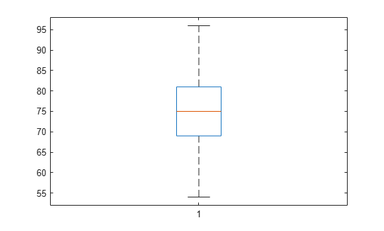
The top line of the box shows the 75th percentile, and the bottom line shows the 25th percentile. The center line shows the median, which is the 50th percentile.
Input Arguments
Probability distribution, specified as one of the probability distribution objects in the following table.
| Distribution Object | Function or App Used to Create Probability Distribution Object |
|---|---|
BetaDistribution | makedist, fitdist, Distribution Fitter |
BinomialDistribution | makedist, fitdist,
Distribution Fitter |
BirnbaumSaundersDistribution | makedist, fitdist,
Distribution Fitter |
BurrDistribution | makedist, fitdist,
Distribution Fitter |
EmpiricalDistribution | fitdist |
ExponentialDistribution | makedist, fitdist,
Distribution Fitter |
ExtremeValueDistribution | makedist, fitdist,
Distribution Fitter |
GammaDistribution | makedist, fitdist,
Distribution Fitter |
GeneralizedExtremeValueDistribution | makedist, fitdist,
Distribution Fitter |
GeneralizedParetoDistribution | makedist, fitdist,
Distribution Fitter |
HalfNormalDistribution | makedist, fitdist,
Distribution Fitter |
InverseGaussianDistribution | makedist, fitdist,
Distribution Fitter |
KernelDistribution | fitdist, Distribution Fitter |
LogisticDistribution | makedist, fitdist,
Distribution Fitter |
LoglogisticDistribution | makedist, fitdist,
Distribution Fitter |
LognormalDistribution | makedist, fitdist,
Distribution Fitter |
LoguniformDistribution | makedist |
MultinomialDistribution | makedist |
NakagamiDistribution | makedist, fitdist,
Distribution Fitter |
NegativeBinomialDistribution | makedist, fitdist,
Distribution Fitter |
NormalDistribution | makedist, fitdist,
Distribution Fitter |
PearsonDistribution | makedist |
PiecewiseLinearDistribution | makedist |
PoissonDistribution | makedist, fitdist,
Distribution Fitter |
RayleighDistribution | makedist, fitdist,
Distribution Fitter |
RicianDistribution | makedist, fitdist,
Distribution Fitter |
StableDistribution | makedist, fitdist,
Distribution Fitter |
tLocationScaleDistribution | makedist, fitdist,
Distribution Fitter |
TriangularDistribution | makedist |
UniformDistribution | makedist |
WeibullDistribution | makedist, fitdist,
Distribution Fitter |
Extended Capabilities
Usage notes and limitations:
The input argument
pdcan be a fitted probability distribution object for beta, exponential, extreme value, lognormal, normal, and Weibull distributions. Createpdby fitting a probability distribution to sample data from thefitdistfunction. For an example, see Code Generation for Probability Distribution Objects.
For more information on code generation, see Introduction to Code Generation and General Code Generation Workflow.
This function fully supports GPU arrays. For more information, see Run MATLAB Functions on a GPU (Parallel Computing Toolbox).
Version History
Introduced in R2013a
MATLAB Command
You clicked a link that corresponds to this MATLAB command:
Run the command by entering it in the MATLAB Command Window. Web browsers do not support MATLAB commands.
Sélectionner un site web
Choisissez un site web pour accéder au contenu traduit dans votre langue (lorsqu'il est disponible) et voir les événements et les offres locales. D’après votre position, nous vous recommandons de sélectionner la région suivante : .
Vous pouvez également sélectionner un site web dans la liste suivante :
Comment optimiser les performances du site
Pour optimiser les performances du site, sélectionnez la région Chine (en chinois ou en anglais). Les sites de MathWorks pour les autres pays ne sont pas optimisés pour les visites provenant de votre région.
Amériques
- América Latina (Español)
- Canada (English)
- United States (English)
Europe
- Belgium (English)
- Denmark (English)
- Deutschland (Deutsch)
- España (Español)
- Finland (English)
- France (Français)
- Ireland (English)
- Italia (Italiano)
- Luxembourg (English)
- Netherlands (English)
- Norway (English)
- Österreich (Deutsch)
- Portugal (English)
- Sweden (English)
- Switzerland
- United Kingdom (English)