fourier

Fourier transform of symbolic expression or function

Syntax

FT = fourier(f)

FT = fourier(f,transVar)

FT = fourier(f,var,transVar)

Description

FT = fourier(f) returns the Fourier transform of f. By default, the function symvar determines the independent variable, and w is the transformation variable.

FT = fourier(f,transVar) uses the transformation variable transVar instead of w.

FT = fourier(f,var,transVar) uses the independent variable var and the transformation variable transVar instead of symvar(f,1) and w, respectively.

Examples

Fourier Transform of Common Functions

Compute the Fourier transform of common functions. By default, the transform is in terms of w.

Find the Fourier transform of a rectangular pulse function.

syms a b t
f = rectangularPulse(a,b,t);
FT = fourier(f)

FT = 
$$-\frac{\sin \left(a\hspace{0.17em}w\right)+\cos \left(a\hspace{0.17em}w\right)\hspace{0.17em}\mathrm{i}}{w}+\frac{\sin \left(b\hspace{0.17em}w\right)+\cos \left(b\hspace{0.17em}w\right)\hspace{0.17em}\mathrm{i}}{w}$$

Find the Fourier transform of a unit impulse (Dirac delta function).

f = dirac(t);
FT = fourier(f)

FT = $$1$$

Find the Fourier transform of the absolute value function.

f = a*abs(t);
FT = fourier(f)

FT = 
$$-\frac{2\hspace{0.17em}a}{w^2}$$

Find the Fourier transform of the step function (Heaviside function).

f = heaviside(t);
FT = fourier(f)

FT = 
$$\pi \hspace{0.17em}\delta \text{<a href="matlab:doc symbolic/dirac">dirac</a>}\left(w\right)-\frac{\mathrm{i}}{w}$$

Find the Fourier transform of a constant.

f = a;
FT = fourier(f)

FT = $$2\hspace{0.17em}\pi \hspace{0.17em}{\delta \text{<a href="matlab:doc symbolic/dirac">dirac</a>}}^{\prime }\left(w\right)\hspace{0.17em}\mathrm{i}$$

Find the Fourier transform of the cosine function.

f = a*cos(b*t);
FT = fourier(f)

FT = $$\pi \hspace{0.17em}a\hspace{0.17em}\left(\delta \text{<a href="matlab:doc symbolic/dirac">dirac</a>}\left(b+w\right)+\delta \text{<a href="matlab:doc symbolic/dirac">dirac</a>}\left(b-w\right)\right)$$

Find the Fourier transform of the sine function.

f = a*sin(b*t);
FT = fourier(f)

FT = $$\pi \hspace{0.17em}a\hspace{0.17em}\left(\delta \text{<a href="matlab:doc symbolic/dirac">dirac</a>}\left(b+w\right)-\delta \text{<a href="matlab:doc symbolic/dirac">dirac</a>}\left(b-w\right)\right)\hspace{0.17em}\mathrm{i}$$

Find the Fourier transform of the sign function.

f = sign(t);
FT = fourier(f)

FT = 
$$-\frac{2\hspace{0.17em}\mathrm{i}}{w}$$

Find the Fourier transform of the right-sided exponential function without any assumptions.

f = exp(-t*abs(a))*heaviside(t);
FT = fourier(f)

FT = 
$$\frac{1}{\left|a\right|+w\hspace{0.17em}\mathrm{i}}-\left(\frac{\mathrm{sign}\left(\left|a\right|\right)}{2}-\frac{1}{2}\right)\hspace{0.17em}\mathrm{fourier}\left({\mathrm{e}}^{-t\hspace{0.17em}\left|a\right|},t,w\right)$$

Find the Fourier transform of the right-sided exponential function, assuming that a > 0. Clear the assumption after computing the Fourier transform.

assume(a > 0)
FTwithAssumption = fourier(f)

FTwithAssumption = 
$$\frac{1}{a+w\hspace{0.17em}\mathrm{i}}$$

assume(a,"clear")

Find the Fourier transform of the double-sided exponential function, assuming that a > 0. Clear the assumption after computing the Fourier transform.

assume(a > 0)
f = exp(-a*t^2);
FTwithAssumption = fourier(f)

FTwithAssumption = 
$$\frac{\sqrt{\pi }\hspace{0.17em}{\mathrm{e}}^{-\frac{w^2}{4\hspace{0.17em}a}}}{\sqrt{a}}$$

assume(a,"clear")

Find the Fourier transform of a Gaussian function, assuming that b and c are real. Simplify the result and clear the assumptions after computing the Fourier transform.

syms c
assume([b c],"real")
f = a*exp(-(t-b)^2/(2*c^2));
FT = fourier(f);
FTsimplified = simplify(FT)

FTsimplified = 
$$\sqrt{2}\hspace{0.17em}a\hspace{0.17em}\sqrt{\pi }\hspace{0.17em}{\mathrm{e}}^{-\frac{w\hspace{0.17em}\left(w\hspace{0.17em}{c}^2+2\hspace{0.17em}b\hspace{0.17em}\mathrm{i}\right)}{2}}\hspace{0.17em}\left|c\right|$$

assume([b c],"clear")

Find the Fourier transform of the Bessel function of the first kind with nu = 1. Simplify the result.

syms x
f = besselj(1,x);
FT = fourier(f);
FTsimplified = simplify(FT)

FTsimplified = 
$$-\frac{2\hspace{0.17em}w\hspace{0.17em}\mathrm{rectangularPulse}\left(-1,1,-w\right)\hspace{0.17em}\mathrm{i}}{\sqrt{1-w^2}}$$

Specify Independent and Transformation Variables

Find the Fourier transform of exp(-t^2-x^2). By default, symvar determines the independent variable, and w is the transformation variable. Here, symvar chooses x.

syms t x
f = exp(-t^2-x^2);
FT = fourier(f)

FT = 
$$\sqrt{\pi }\hspace{0.17em}{\mathrm{e}}^{-t^2-\frac{w^2}{4}}$$

Specify the transformation variable as y. If you specify only one variable, that variable is the transformation variable. symvar still determines the independent variable.

syms y
FT = fourier(f,y)

FT = 
$$\sqrt{\pi }\hspace{0.17em}{\mathrm{e}}^{-t^2-\frac{y^2}{4}}$$

Specify the independent and transformation variables as t and y, respectively.

FT = fourier(f,t,y)

FT = 
$$\sqrt{\pi }\hspace{0.17em}{\mathrm{e}}^{-x^2-\frac{y^2}{4}}$$

Plot Rectangular Pulse and Its Fourier Transform

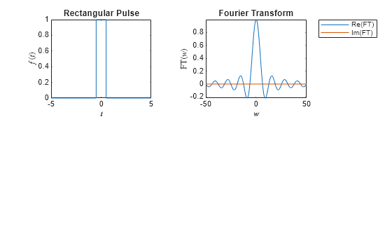
Create a rectangular pulse with a starting point at –1/2 and an endpoint at 1/2.

syms t
f1 = rectangularPulse(-1/2,1/2,t);

Find its Fourier transform. Simplify the result. Here, the Fourier transform contains only the real part.

FT1 = fourier(f1);
FT1 = simplify(FT1)

FT1 = 
$$\frac{2\hspace{0.17em}\sin \left(\frac{w}{2}\right)}{w}$$

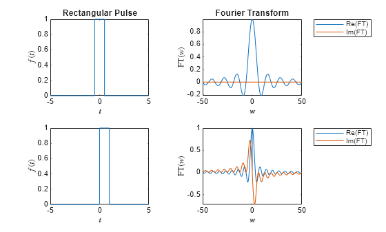
Plot the rectangular pulse in a 2-by-2 tiled chart layout by using fplot. Plot the real and imaginary parts of its Fourier transform.

tiledlayout(2,2)

nexttile
fplot(f1)
xlabel("$t$",Interpreter="latex")
ylabel("$f(t)$",Interpreter="latex")
title("Rectangular Pulse")

nexttile
fplot(real(FT1),[-50 50])
hold on
fplot(imag(FT1),[-50 50])
xlabel("$w$",Interpreter="latex")
ylabel("FT($w$)",Interpreter="latex")
title("Fourier Transform")
legend("Re(FT)","Im(FT)",Location="northeastoutside")

Next, create another rectangular pulse with a starting point at 0 and an endpoint at 1.

f2 = rectangularPulse(0,1,t);

Find its Fourier transform. Here, the Fourier transform contains both real and imaginary parts.

FT2 = fourier(f2)

FT2 = 
$$\frac{\sin \left(w\right)+\cos \left(w\right)\hspace{0.17em}\mathrm{i}}{w}-\frac{\mathrm{i}}{w}$$

Plot the rectangular pulse. Plot the real and imaginary parts of its Fourier transform.

nexttile
fplot(f2)
xlabel("$t$",Interpreter="latex")
ylabel("$f(t)$",Interpreter="latex")

nexttile
fplot(real(FT2),[-50 50])
hold on
fplot(imag(FT2),[-50 50])
xlabel("$w$",Interpreter="latex")
ylabel("FT($w$)",Interpreter="latex")
legend("Re(FT)","Im(FT)",Location="northeastoutside")

Fourier Transforms Involving Dirac and Heaviside Functions

Find the Fourier transform of t^3. The result is in terms of the third derivative of the Dirac delta function.

syms t w
FT = fourier(t^3,t,w)

FT = $$-2\hspace{0.17em}\pi \hspace{0.17em}{\delta \text{<a href="matlab:doc symbolic/dirac">dirac</a>}}^{\prime \prime \prime }\left(w\right)\hspace{0.17em}\mathrm{i}$$

Find the Fourier transform of the Heaviside function with a discontinuity at t0.

syms t0
FT = fourier(heaviside(t - t0),t,w)

FT = 
$${\mathrm{e}}^{-t_0\hspace{0.17em}w\hspace{0.17em}\mathrm{i}}\hspace{0.17em}\left(\pi \hspace{0.17em}\delta \text{<a href="matlab:doc symbolic/dirac">dirac</a>}\left(w\right)-\frac{\mathrm{i}}{w}\right)$$

Specify Fourier Transform Parameters

As described in the More About section, $$c$$ and $$s$$ are parameters of the Fourier transform. By default, the fourier function uses $$c=1$$ and $$s=-1$$. However, you can change those parameter values by using sympref.

Compute the Fourier transform of t*exp(-t^2) using the default values of the Fourier parameters.

syms t w
f = t*exp(-t^2);
FT = fourier(f,t,w)

FT = 
$$-\frac{w\hspace{0.17em}\sqrt{\pi }\hspace{0.17em}{\mathrm{e}}^{-\frac{w^2}{4}}\hspace{0.17em}\mathrm{i}}{2}$$

Change the Fourier parameters to c = 1 and s = 1 by using sympref, and compute the transform again. The result changes.

sympref("FourierParameters",[1 1]);
FT = fourier(f,t,w)

FT = 
$$\frac{w\hspace{0.17em}\sqrt{\pi }\hspace{0.17em}{\mathrm{e}}^{-\frac{w^2}{4}}\hspace{0.17em}\mathrm{i}}{2}$$

Change the Fourier parameters to c = 1/(2*pi) and s = 1, and compute the transform again. The result changes.

sympref("FourierParameters",[1/(2*sym(pi)) 1]);
FT = fourier(f,t,w)

FT = 
$$\frac{w\hspace{0.17em}{\mathrm{e}}^{-\frac{w^2}{4}}\hspace{0.17em}\mathrm{i}}{4\hspace{0.17em}\sqrt{\pi }}$$

Symbolic settings that you set using sympref persist through your current and future MATLAB® sessions. Restore the default values of c and s by setting FourierParameters to "default".

sympref("FourierParameters","default");

Fourier Transform Using Array Inputs

Find the Fourier transform of the matrix M. Specify the independent and transformation variables for each matrix element by using matrices of the same size. When the arguments are nonscalar, fourier acts on them element-wise.

syms a b c d w x y z
M = [exp(x) 1; sin(y) 1i*z];
vars = [w x; y z];
transVars = [a b; c d];
FT = fourier(M,vars,transVars)

FT = 
$$\left(\begin{array}{cc}2\hspace{0.17em}\pi \hspace{0.17em}{\mathrm{e}}^x\hspace{0.17em}\delta \text{<a href="matlab:doc symbolic/dirac">dirac</a>}\left(a\right)& 2\hspace{0.17em}\pi \hspace{0.17em}\delta \text{<a href="matlab:doc symbolic/dirac">dirac</a>}\left(b\right)\\ -\pi \hspace{0.17em}\left(\delta \text{<a href="matlab:doc symbolic/dirac">dirac</a>}\left(c-1\right)-\delta \text{<a href="matlab:doc symbolic/dirac">dirac</a>}\left(c+1\right)\right)\hspace{0.17em}\mathrm{i}& -2\hspace{0.17em}\pi \hspace{0.17em}{\delta \text{<a href="matlab:doc symbolic/dirac">dirac</a>}}^{\prime }\left(d\right)\end{array}\right)$$

If you call fourier with both scalar and nonscalar arguments, then it expands the scalar arguments to match the nonscalar arguments by using scalar expansion. Nonscalar arguments must be the same size.

FT = fourier(x,vars,transVars)

FT = 
$$\left(\begin{array}{cc}2\hspace{0.17em}\pi \hspace{0.17em}x\hspace{0.17em}\delta \text{<a href="matlab:doc symbolic/dirac">dirac</a>}\left(a\right)& 2\hspace{0.17em}\pi \hspace{0.17em}{\delta \text{<a href="matlab:doc symbolic/dirac">dirac</a>}}^{\prime }\left(b\right)\hspace{0.17em}\mathrm{i}\\ 2\hspace{0.17em}\pi \hspace{0.17em}x\hspace{0.17em}\delta \text{<a href="matlab:doc symbolic/dirac">dirac</a>}\left(c\right)& 2\hspace{0.17em}\pi \hspace{0.17em}x\hspace{0.17em}\delta \text{<a href="matlab:doc symbolic/dirac">dirac</a>}\left(d\right)\end{array}\right)$$

Uncomputable Fourier Transform

If fourier cannot transform the input, then it returns an unevaluated call.

syms f(t) w
FT = fourier(f,t,w)

FT = $$\mathrm{fourier}\left(f\left(t\right),t,w\right)$$

Return the original expression by using ifourier.

f = ifourier(FT,w,t)

f = $$f\left(t\right)$$

Two-Dimensional Fourier Transform

Find the 2-D Fourier transform by independently applying a sequence of 1-D Fourier transforms to each of the independent variables.

In this example, set the Fourier parameters to $$c=1$$ and $$s=2\pi$$ such that the formula for the 2-D Fourier transform is

$\mathit{F}\left(\mathit{u},\mathit{v}\right)={\int }_{-\infty }^{\infty }{\int }_{-\infty }^{\infty }\mathit{f}\left(\mathit{x},\mathit{y}\right){\mathit{e}}^{\mathit{i}\left(\mathit{2}\pi \mathrm{ux}+\mathit{2}\pi \mathrm{vy}\right)}\mathit{dx}\mathit{dy}$.

You can specify these parameters by using sympref.

sympref("FourierParameters",[1 2*sym(pi)]);

Find the 2-D Fourier transform of a 2-D unit rectangle located at the origin with width a and height b. Perform the 1-D Fourier transforms on the variable $$x$$, followed by the variable $$y$$. Simplify the result.

syms x y a b real
f(x,y) = rectangularPulse(-a/2,a/2,x)*rectangularPulse(-b/2,b/2,y);
syms u v
FT = fourier(f,x,u);
FT = fourier(FT,y,v);
FT = simplify(FT)

FT = 
$$\frac{\sin \left(\pi \hspace{0.17em}a\hspace{0.17em}u\right)\hspace{0.17em}\sin \left(\pi \hspace{0.17em}b\hspace{0.17em}v\right)}{u\hspace{0.17em}v\hspace{0.17em}{\pi }^2}$$

Find the Fourier transform of a 2-D Gaussian function with standard deviation $$\sigma$$ in both the $$x$$- and $$y$$-directions.

syms sigma real
f(x,y) = 1/2/sym(pi)/sigma^2*exp((-x^2-y^2)/2/sigma^2);
syms u v
FT = fourier(f,x,u);
FT = fourier(FT,y,v);
FT = simplify(FT)

FT = $${\mathrm{e}}^{-2\hspace{0.17em}{\sigma }^2\hspace{0.17em}{\pi }^2\hspace{0.17em}\left(u^2+v^2\right)}$$

Find the Fourier transform of two point sources located at $$(x,y)=(0,a)$$ and $$(x,y)=(0,-a)$$.

f(x,y) = 1/2*dirac(x)*(dirac(y-a)+dirac(y+a));
FT = fourier(f,x,u);
FT = fourier(FT,y,v);
FT = simplify(FT)

FT = $$\cos \left(2\hspace{0.17em}\pi \hspace{0.17em}a\hspace{0.17em}v\right)$$

Find the Fourier transform of a unit circle aperture. Define the unit circle by using the heaviside function.

f(x,y) = heaviside(x^2+y^2-1);
FT = fourier(f,x,u);
FT = fourier(FT,y,v)

FT = $$\mathrm{fourier}\left(\mathrm{fourier}\left(\mathrm{heaviside}\left(x^2+y^2-1\right),x,u\right),y,v\right)$$

Here, the fourier function cannot transform the input function and returns an unevaluated call. As an alternative, you can find the 2-D Fourier transform numerically by using the fft2 function. For an example of how to find the 2-D Fourier transform of a circular aperture, see 2-D Fourier Transforms.

Symbolic settings that you set using sympref persist through your current and future MATLAB sessions. Restore the default settings.

sympref("default");

Input Arguments

f — Input

symbolic expression | symbolic function | symbolic vector | symbolic matrix

Input, specified as a symbolic expression, function, vector, or matrix.

transVar — Transformation variable

w (default) | v | symbolic variable | symbolic expression | symbolic vector | symbolic matrix

Transformation variable, specified as a symbolic variable, expression, vector, or matrix. This variable is often referred to as the "frequency variable." By default, fourier uses w. If w is the independent variable of f, then fourier uses v.

var — Independent variable

symvar of f (default) | symbolic variable | symbolic vector | symbolic matrix

Independent variable, specified as a symbolic variable, vector, or matrix. This variable is often referred to as the "time variable" or the "space variable." If you do not specify this argument, then fourier uses the function symvar(f,1) to determine the independent variable.

More About

Fourier Transform

The Fourier transform of the expression f = f(x) with respect to the variable x at the point w is

$$F\left(w\right)=c{\displaystyle \underset{-\infty }{\overset{\infty }{\int }}f\left(x\right)e^{iswx}dx},$$

where c and s are parameters of the Fourier transform. The fourier function uses c = 1 and s = –1.

Tips

• If any argument is an array, then fourier acts element-wise on all elements of the array.

• If the first argument contains a symbolic function, then the second argument must be a scalar.

• To compute the inverse Fourier transform, use ifourier.

• fourier does not transform piecewise. Instead, try to rewrite piecewise by using the functions heaviside, rectangularPulse, or triangularPulse.

References

[1] Oberhettinger, Fritz. Tables of Fourier Transforms and Fourier Transforms of Distributions. Berlin, Heidelberg: Springer Berlin Heidelberg, 1990.

Version History

Introduced before R2006a