Automatically Tune Quadcopter PID Gains to Reduce Mission Time

R2026b

This example shows how to automatically tune a cascaded quadcopter flight controller to improve tracking performance and reduce the time required to complete a waypoint mission. This example uses Closed‑Loop PID Autotuner blocks to tune multiple control loops, then compares baseline and tuned mission results.

Getting Started

To get started, open the scdUAVPIDAutotuning project file. The project sets up the workspace, configures the model variants, and provides shortcuts for simulating the baseline mission and running the autotuning mission.

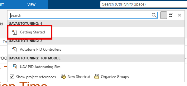
prj = openProject('scdUAVPIDAutotuning');

To set up a high‑fidelity quadcopter plant and initialize a four‑waypoint mission, on the Project tab of the MATLAB Toolstrip, in the Shortcuts section, click the Getting Started shortcut.

Model Overview

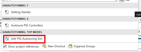
Launching the scdUAVPIDAutotuning project opens the uavPIDAutotuning Simulink® model. If you need to reopen the model, click the UAV PID Autotuning Sim shortcut.

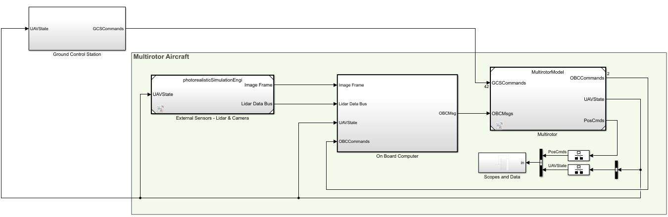
The model simulates a quadcopter that uses a cascaded PID flight controller. It includes vehicle dynamics, guidance logic, sensing, and feedback control loops for position, velocity, attitude, and angular‑rate control.

The top model consists of the following subsystems:

• Ground Control Station — Sends mission commands and monitors UAV state during simulation.

• External Sensors – Lidar & Camera — Interfaces with simulated perception sources.

• On Board Computer — Executes mission‑level logic.

• Multirotor — Implements the quadcopter dynamics and flight controller.

Model parameters and design data are stored in the data dictionary uavPackageDeliveryDataDict.sldd.

Quadcopter Controller Subsystem Overview

Open the Controller subsystem that is located inside of the Multirotor subsystem.

blockpath = Simulink.BlockPath("MultirotorModel/Inner Loop and Plant Model/High-FidelityModel/Control System/Controller");
open(blockpath)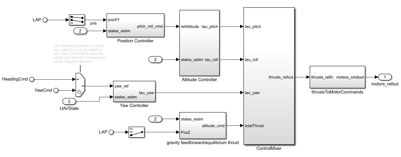

The Controller subsystem contains position, yaw, and attitude controllers. This example focuses on tuning the position and attitude control loops.

Position Controller

The Position Controller subsystem computes pitch and roll setpoints from position‑tracking errors and passes the pitch and roll setpoints to the Attitude Controller subsystem. Within the Position Controller subsystem, a proportional position controller generates velocity setpoints, which are then used by a proportional–integral velocity controller to compute the pitch and roll setpoints.

The baseline gains for this subsystem are:

• X position — Kp = 0.0625

• Y position — Kp = 0.0625

• X velocity — Kp = 0.0375, Ki = 0.01875

• Y velocity — Kp = 0.0375, Ki = 0.01875

Attitude Controller

The Attitude Controller subsystem computes torque commands from attitude tracking errors and passes the torque commands to the ControlMixer subsystem. Within the Attitude Controller subsystem, a proportional angle controller generates angular rate setpoints, which are then used by a PID angular rate controller to compute the torque commands.

The baseline gains for this subsystem are:

• Pitch angle — Kp = 1.25

• Roll angle — Kp = 1.25

• Pitch rate — Kp = 0.000625, Ki = 0.0013, Kd = 0.000025

• Roll rate — Kp = 0.0005, Ki = 0.0008, Kd = 0.000015

Run Mission with Baseline Gains

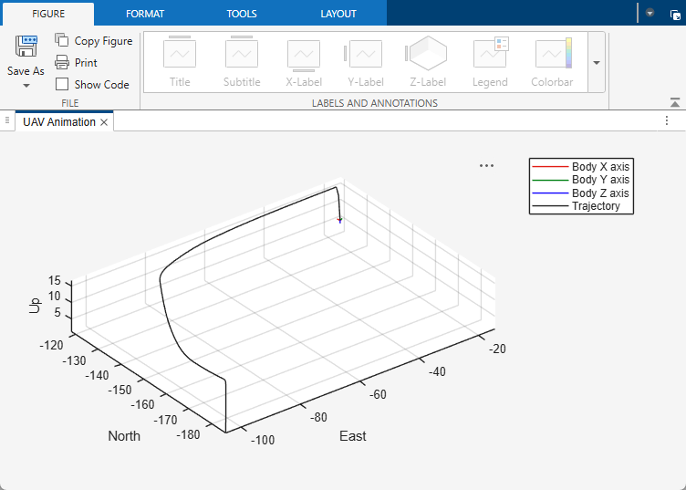
To simulate the quadcopter mission with four waypoints using the baseline gains, run the uavPIDAutotuning Simulink model. The model opens the UAV animation output during simulation using the UAV Animation block. With the baseline controller gains, the quadcopter takes approximately 150 seconds to complete the mission.

Set Up Model for Autotuning

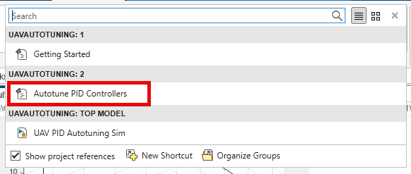
Click the Autotune PID Controllers project shortcut, which sets up the uavPIDAutotuning model to hover at a low altitude, automatically tune the controller gains, and then run the same four‑waypoint mission.

The model contains eight PID control loops organized into four controller layers: attitude rate, attitude, velocity, and position. Closed-Loop PID Autotuner (Simulink Control Design) blocks inject perturbation signals at the output of each PID controller and use closed‑loop feedback to update the controller gains.

This diagram shows how the eight controllers are connected to the Closed‑Loop PID Autotuner blocks during the autotuning process.

Setting Autotuner Blocks

The Closed‑Loop PID Autotuner blocks automatically tune controller gains to achieve specified bandwidth and phase‑margin targets using a closed‑loop experiment. During autotuning, the plant remains under control of the existing controllers while the Closed‑Loop PID Autotuner blocks inject small perturbation signals, estimate the frequency response, and update the controller gains to meet the specified targets.

Bandwidth and Phase Margins

Bandwidth characterizes how quickly a closed‑loop system responds to reference changes and disturbances. It is defined as the frequency at which the closed‑loop magnitude response drops to −3 dB. A higher closed‑loop bandwidth corresponds to a faster rise time and a more responsive controller.

Phase margin characterizes closed‑loop stability and robustness. It is defined as the additional phase lag at the gain crossover frequency (0 dB) required to make the closed‑loop system unstable. In this example, all control loops target a 60‑degree phase margin, which provides a good balance between responsiveness and damping.

Bandwidth Selection for Cascaded Control

The control system sampling time is $T_s$= 0.005 s. The Closed‑Loop PID Autotuner requires that the product of bandwidth $\omega$ and sampling time satisfies:

$$\omega T_s\le 0.3$$

This constraint limits the maximum allowable bandwidth to 60 rad/s. In addition, cascaded control architectures requires the inner loops to have higher bandwidth than outer loops to ensure stability. This table summarizes the bandwidth for each loop in this example:

Control Loop	Bandwidth (rad/s)
Attitude rate	50
Attitude	20
Velocity	5
Position	1

Parallel and Sequential Tuning

All control axes are decoupled except for the pitch and roll rate loops. The x‑ and y‑velocity loops are independent, which allows them to be tuned simultaneously and reduces the overall autotuning time. The pitch and roll rate loops are coupled and are therefore tuned sequentially.

This results in the following tuning sequence:

1. Pitch rate.

2. Roll rate.

3. Pitch and roll angles.

4. X and Y velocities.

5. X and Y positions.

Run Autotuning Mission

Run the uavPIDAutotuning model. The quadcopter takes off and starts the tuning process. During the tuning process, the Closed-Loop PID Autotuner blocks injects perturbations to the UAV.

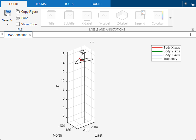
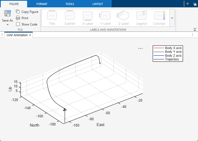
After the autotuning process completes, at approximately 185 seconds into the simulation, the multirotor follows the same four‑waypoint path as in the initial mission but completes the path significantly faster due to the tuned controller gains.

During the autotuning process the gains are updated for the eight controllers:

• X position — Kp = 0.9365

• Y position — Kp = 0.9291

• X velocity — Kp = 0.5153, Ki = 0.2581

• Y velocity — Kp = 0.5201, Ki = 0.2979

• Pitch angle — Kp = 19.38

• Roll angle — Kp = 18.95

• Pitch rate — Kp = 0.00425, Ki = 0.01479, Kd = 0.0000045

• Roll rate — Kp = 0.003477, Ki = 0.01215, Kd = 0.0000031

Comparison of Baseline and Tuned Quadcopter Response

These plots show the position and attitude responses of the quadcopter along the waypoint path. The blue lines represent performance with the baseline controller gains, while the red lines represent performance with the tuned gains. With the tuned gains, the multirotor completes the path in approximately 45 seconds. With the baseline gains, the same path takes nearly 150 seconds.

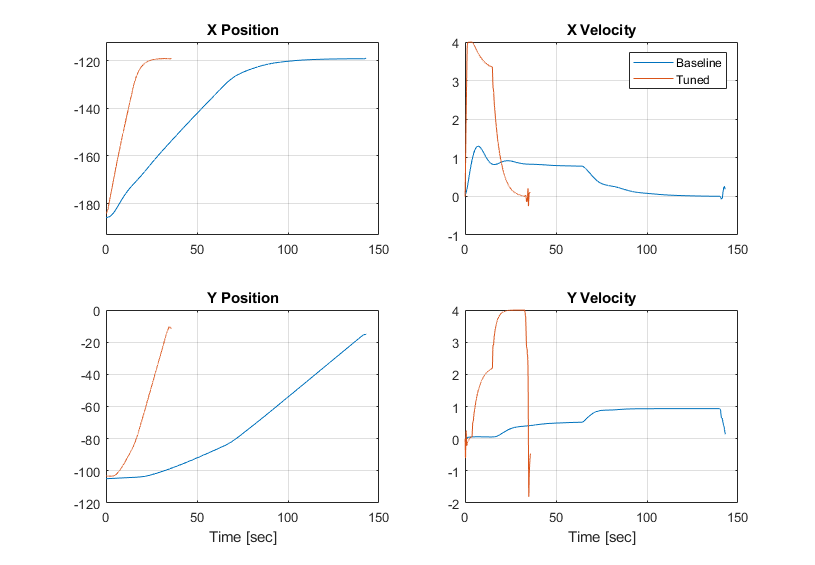
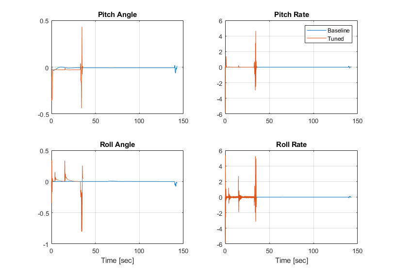
To reproduce the comparison between the baseline and tuned responses, run the quadcopter mission twice. First, run the mission using the original controller gains by clicking the Getting Started project shortcut. Then update the controller gains with the tuned values and run the same four‑waypoint mission again.

In each simulation run, the quadcopter response is stored in the UAVData_out workspace variable, which you can use to compare position, velocity, and attitude responses between the baseline and tuned cases.

When you are done exploring the models, close the project file.

close(prj)