blscalf
Syntax
Description
Examples
Obtain the scaling filter corresponding to the best-localized Daubechies wavelet with 10 vanishing moments. Confirm the sum of the filter coefficients nearly equals and the L2 norm of the filter nearly equals 1.
scalf = blscalf("bl10");
sum(scalf)-sqrt(2)
ans = -2.2204e-16
norm(scalf,2)
ans =
1.0000
Use orthfilt to obtain the scaling and wavelet filters corresponding to the wavelet.
[LoD,HiD,LoR,HiR] = orthfilt(scalf);
Confirm the filters form an orthonormal perfect reconstruction wavelet filter bank.
[tf,checks] = isorthwfb(LoD)
tf = logical
   1
checks=7×3 table
                                          Pass-Fail    Maximum Error    Test Tolerance
                                          _________    _____________    ______________

    Equal-length filters                    pass                 0                 0
    Even-length filters                     pass                 0                 0
    Unit-norm filters                       pass        1.7665e-10        1.4901e-08
    Filter sums                             pass        7.2923e-15        1.4901e-08
    Even and odd downsampled sums           pass        3.7748e-15        1.4901e-08
    Zero autocorrelation at even lags       pass        7.3088e-11        1.4901e-08
    Zero crosscorrelation at even lags      pass        1.3089e-17        1.4901e-08
Create a discrete wavelet transform filter bank using the wavelet. Plot the frequency responses of the wavelet filters and the final resolution scaling filter for the default signal length.
fb = dwtfilterbank(Wavelet="bl10");
freqz(fb)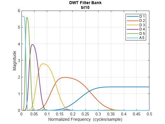
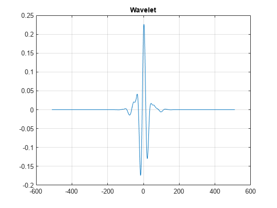
Plot the wavelet at the coarsest scale.
[psi,t] = wavelets(fb);
plot(t,psi(end,:))
grid on
title("Wavelet")
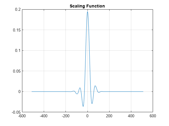
Plot the scaling function at the coarsest scale.
[phi,t] = scalingfunctions(fb);
plot(t,phi(end,:))
grid on
title("Scaling Function")
Input Arguments
Output Arguments
References
[1] Doroslovački, M.L. “On the Least Asymmetric Wavelets.” IEEE Transactions on Signal Processing 46, no. 4 (April 1998): 1125–30. https://doi.org/10.1109/78.668562.
Extended Capabilities
Version History
Introduced in R2022b