Generate Generic C Code for a Human Health Monitoring Network
This example shows how to generate a generic C MEX application for a deep learning network that reconstructs electrocardiogram (ECG) signals from a continuous wave (CW) radar. CW radars are used for daily long-term monitoring and are an alternative to wearable devices, which can monitor ECG signals directly.
To learn about the network and the network training process, see Human Health Monitoring Using Continuous Wave Radar and Deep Learning. This example uses the network that contains a maximal overlap discrete wavelet transform (MODWT) layer.
Download and Prepare Data
The data set [1] in this example contains synchronized data from a CW radar and ECG signals measured simultaneously by a reference device on 30 healthy subjects. The CW radar system uses the six-port technique and operates at 24 GHz in the Industrial Scientific and Medical (ISM) band.
Because the original data set contains a large volume of data, this example uses the data from resting, apnea, and Valsalva maneuver scenarios. Additionally, it uses only the data from subjects 1 through 5 to train and validate the model, and data from subject 6 to test the trained model.
Because the main information in the ECG signal is usually in a frequency band less than 100 Hz, all signals are downsampled to 200 Hz and divided into segments of 1024 points to create signals of approximately 5s.
Download the data set by using the downloadSupportFile function. The whole data set is approximately 16 MB in size and contains two folders. The trainVal folder contains the training and validation data and the test folder contains the test data. Each folder contains ecg and radar folders for ECG and radar signals, respectively.
datasetZipFile = matlab.internal.examples.downloadSupportFile('SPT','data/SynchronizedRadarECGData.zip');
datasetFolder = fullfile(fileparts(datasetZipFile),'SynchronizedRadarECGData');
if ~exist(datasetFolder,'dir')
    unzip(datasetZipFile,datasetFolder);
end
Create signalDatastore objects to access the data in the files. Create datastores radarTrainValDs and radarTestDs to store the CW radar data used for training/validation and testing, respectively. Then create ecgTrainValDs and ecgTestDs datastore objects to store the ECG signals for training/validation and testing, respectively.
radarTrainValDs = signalDatastore(fullfile(datasetFolder,"trainVal","radar"));
radarTestDs = signalDatastore(fullfile(datasetFolder,"test","radar"));
ecgTrainValDs = signalDatastore(fullfile(datasetFolder,"trainVal","ecg"));
ecgTestDs = signalDatastore(fullfile(datasetFolder,"test","ecg"));
View the categories and distribution of the training data.
trainCats = filenames2labels(radarTrainValDs,'ExtractBefore','_radar');
summary(trainCats)
trainCats: 830×1 categorical

     GDN0001_Resting        59
     GDN0001_Valsalva       97
     GDN0002_Resting        60
     GDN0002_Valsalva       97
     GDN0003_Resting        58
     GDN0003_Valsalva      103
     GDN0004_Apnea          14
     GDN0004_Resting        58
     GDN0004_Valsalva      106
     GDN0005_Apnea          14
     GDN0005_Resting        59
     GDN0005_Valsalva      105
     <undefined>             0
View the categories and distribution of the test data.
testCats = filenames2labels(radarTestDs,'ExtractBefore','_radar');
summary(testCats)
testCats: 200×1 categorical

     GDN0006_Apnea          14
     GDN0006_Resting        59
     GDN0006_Valsalva      127
     <undefined>             0
Apply normalization to the ECG signals. Use the helperNormalize helper function to center each signal by subtracting its median and rescale it so that its maximum peak is 1.
ecgTrainValDs = transform(ecgTrainValDs,@helperNormalize);
ecgTestDs = transform(ecgTestDs,@helperNormalize);
Combine the data sets into a training and a test data set.
trainValDs = combine(radarTrainValDs,ecgTrainValDs);
testDs = combine(radarTestDs,ecgTestDs);
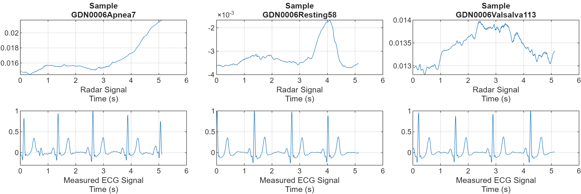
Visualize the CW radar and measured ECG signals for one of each of the scenarios. The deep learning network takes the radar signal and reconstructs it to the corresponding ECG signal.
numCats = cumsum(countcats(testCats));
previewindices = [randi([1,numCats(1)]),randi([numCats(1)+1,numCats(2)]),randi([numCats(2)+1,numCats(3)])];
testindices = [randi([1,numCats(1)]),randi([numCats(1)+1,numCats(2)]),randi([numCats(2)+1,numCats(3)])];

helperPlotData(testDs,previewindices);
Inspect the Entry-Point Function
The radarToEcgNet_predict entry-point function loads the dlnetwork object from the radarToEcgNet MAT file into a persistent variable and reuses the variable for subsequent prediction calls. The entry-point function converts the input CW radar data into a dlarray format and calls the predict method on the network by using the dlarray input data. Finally, it reshapes the output into a two-dimensional array.
type('radarToEcgNet_predict.m')function out = radarToEcgNet_predict(in) %#codegen
% Copyright 2024 The MathWorks, Inc.
persistent dlnet
if isempty(dlnet)
dlnet = coder.loadDeepLearningNetwork('radarToEcgNet.mat');
end
% convert input to a dlarray
dlIn = dlarray(single(in),'CTB');
% pass in input
dlOut = predict(dlnet,dlIn);
% extract data from dlarray and reshape it to two dimensions
out = extractdata(dlOut);
out = reshape(out, [1,numel(dlOut)]);
end
Configure Code Generation Options and Generate Code
Create a code generation configuration object by using the coder.config (MATLAB Coder) function. For the cfg object, the default value of DeepLearningConfig is a coder.DeepLearningCodeConfig (MATLAB Coder) object. By default, the generated code does not depend on any third-party deep learning libraries.
cfg = coder.config('mex');
cfg.DeepLearningConfig
ans =
coder.DeepLearningCodeConfig with properties:
TargetLibrary: 'none'
------------------- CPU optimizations -------------------
LearnablesCompression: 'None'
------------------- GPU optimizations -------------------
ComputePrecision: 'FP32'
Because the network requires the CW radar data as an input argument, prepare a sample CW radar data for code generation.
exampleRadarData = read(radarTrainValDs);
Run the codegen command. Specify the sample data as the input type.
codegen radarToEcgNet_predict -config cfg -args {exampleRadarData}
Code generation successful.
Run the Generated MEX Function
Run the generated MEX function by passing a CW radar signal.
idx = testindices(1);
ds = subset(radarTestDs,idx);
testRadarData = read(ds);
predictedEcg_mex = radarToEcgNet_predict_mex(testRadarData);
Run the entry-point function in MATLAB to compare the results.
predictedEcg = radarToEcgNet_predict(testRadarData);
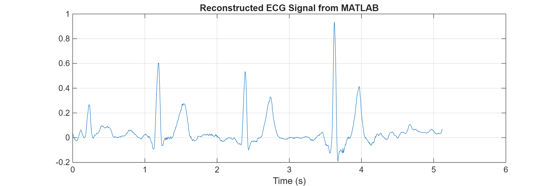
Plot the data.
tiledlayout(1, 2, 'Padding', 'none', 'TileSpacing', 'compact');

fs = 200;
t = linspace(0,length(predictedEcg)/fs,length(predictedEcg));

plot(t,predictedEcg)
title("Reconstructed ECG Signal from MATLAB")
xlabel("Time (s)")
grid on

nexttile(2)
plot(t,predictedEcg_mex)
title("Reconstructed ECG Signal from Generated MEX")
xlabel("Time (s)")
grid on
The reconstructed ECG signals from MATLAB and the generated MEX function match.
Compare Predicted Signals to the Measured ECG Signals
Visualize the output of the deep learning network for all three input signal scenarios and compare it to the measured ECG signal data. To do this, call the helper function helperPlotData by passing the generated MEX function, radarToEcgNet_predict_mex, as a function handle. The helper function picks a representative input for each scenario, runs the generated MEX with that data, and visualizes the result alongside the corresponding measured ECG signal.
helperPlotData(testDs,testindices,@radarToEcgNet_predict_mex);
Reference
[1] Schellenberger, S., Shi, K., Steigleder, T. et al. A data set of clinically recorded radar vital signs with synchronized reference sensor signals. Sci Data 7, 291 (2020). https://doi.org/10.1038/s41597-020-00629-5
Helper Functions
The helperNormalize function normalizes input signals by subtracting the median and dividing the signals by the maximum value.
function x = helperNormalize(x)
% This function is only intended to support this example. It may be changed
% or removed in a future release.
    x = x-median(x);
    x = {x/max(x)};
end
The helperPlotData function plots the radar and ECG signals.
function  helperPlotData(DS,Indices,mexFunction)
% This function is only intended to support this example. It may be changed
% or removed in a future release.
    arguments
       DS
       Indices
       mexFunction = []
    end
    fs = 200;
    N = numel(Indices);
    M = 2;
    if ~isempty(mexFunction)
        M = M + 1;
    end

    tiledlayout(M, N, 'Padding', 'none', 'TileSpacing', 'compact');
    for i = 1:N
        idx = Indices(i);
        ds = subset(DS,idx);
        [~,name,~] = fileparts(ds.UnderlyingDatastores{1}.Files{1});
        data = read(ds);
        radar = data{1};
        ecg = data{2};
        t = linspace(0,length(radar)/fs,length(radar));

        nexttile(i)
        plot(t,radar)
        title(["Sample",regexprep(name, {'_','radar'}, '')])
        xlabel(["Radar Signal","Time (s)"])
        grid on

        nexttile(N+i)
        plot(t,ecg)
        xlabel(["Measured ECG Signal","Time (s)"])
        ylim([-0.3,1])
        grid on

        if ~isempty(mexFunction)
            nexttile(2*N+i)
            predictedEcg = mexFunction(radar);
            plot(t,predictedEcg)
            grid on
            ylim([-0.3,1])
            xlabel(["Reconstructed ECG Signal from Generated MEX","Time (s)"])
        end
    end
    set(gcf,'Position',[0 0 300*N,150*M])
end