Antenna Model Generation and Full-Wave Analysis From Photo
This example shows the process of using a photograph of a planar antenna to generate a viable antenna model and its subsequent analysis for port, surface and field characteristics. The Image Segmenter app is used to perform segmentation on the image of an RFID tag, and the resulting boundaries are used to set up the antenna model in Antenna Toolbox™. An initial impedance analysis is done over a frequency range to understand the port characteristics of the antenna. After determining the resonant frequency, the current and far-field pattern are calculated and plotted.
RFID Tag
Begin by taking a photo of an RFID tag against a high-color contrast background. The camera is positioned directly over the antenna. This photo was taken with a smartphone.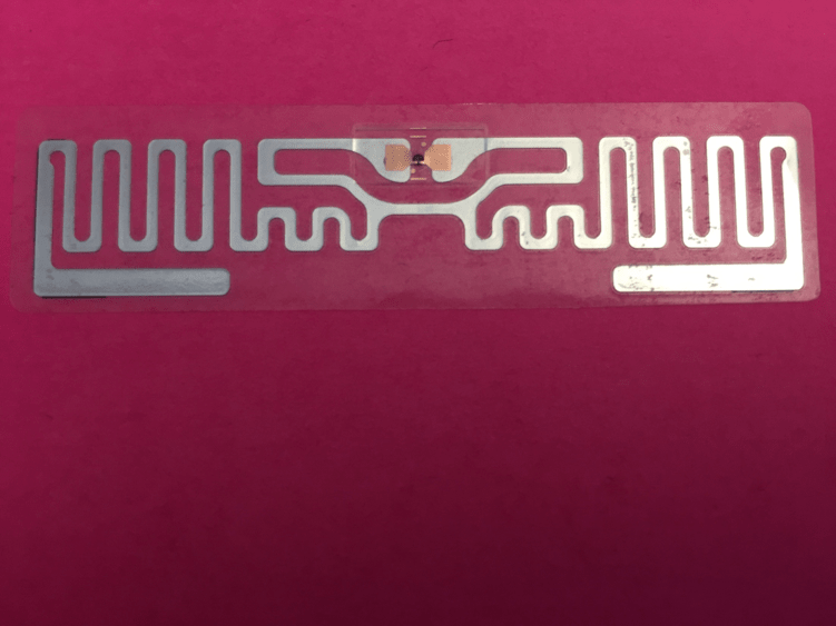
Image Segmentation Using Image Segmenter App
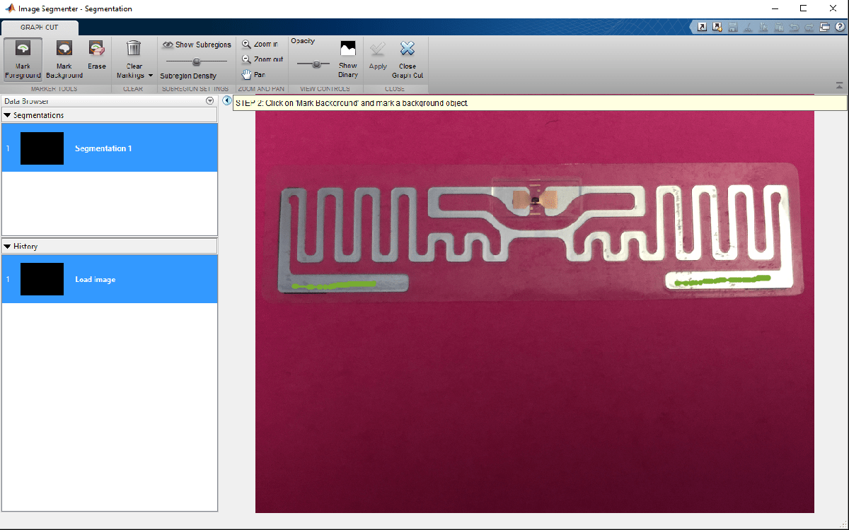
Choose Foreground and Background
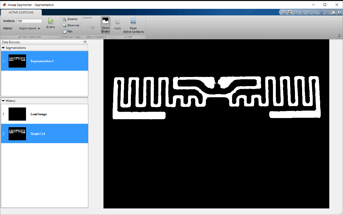
Using the app, import this antenna and choose the graph cut option on the toolstrip. Pick the foreground and background regions on the image. For this example, the foreground region is the metallized regions of the RFID tag and the background is the colored region.
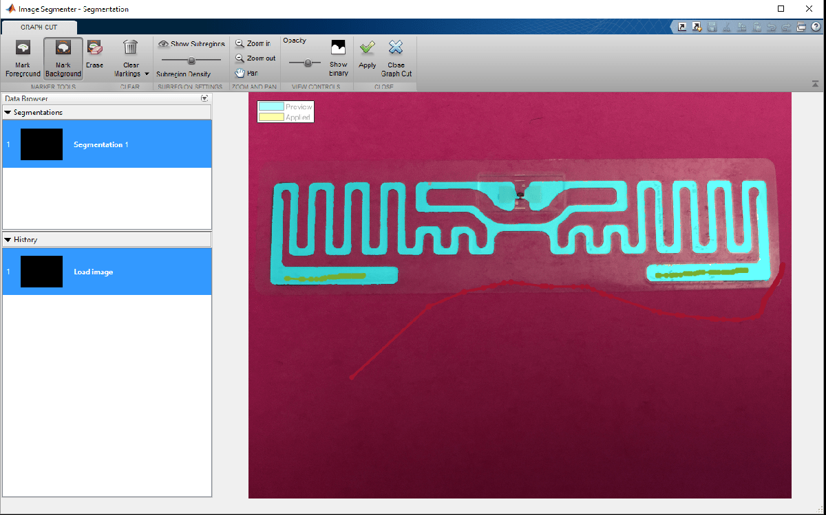
Improve Segmentation Quality
Choosing the background in the app results in an initial segmentation of the image into the foreground and background portions. If this segmentation is sufficient, apply the changes and proceed to the next part of the process by closing the graph cut tab.
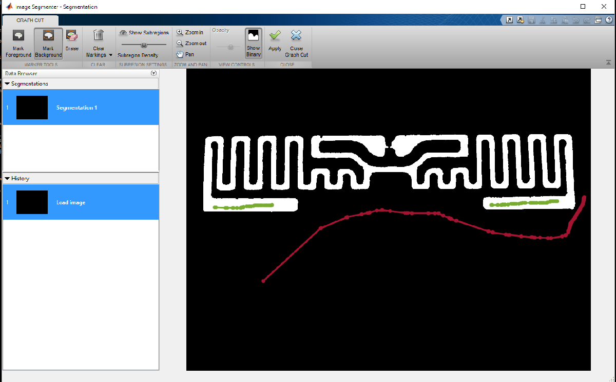
If however, all parts of the antenna have not been identified yet, continue marking up the foreground and background regions. This allows the segmentation algorithm to improve upon the results. It may also be of use to adjust the sub-region density to refine the quality of segmentation. After making the required adjustments, apply the changes and close the graph-cut segmentation tab in the app. On returning to the main tab, there are several options to further improve the segmentation. In this example we use the Active Contours option and evolve the existing segmentation to fill in any imperfections in the boundaries.
Notice that after several iterations of the active contours algorithm has executed, the boundary is much smoother and free of notch like artifacts. An example region is shown for comparison.

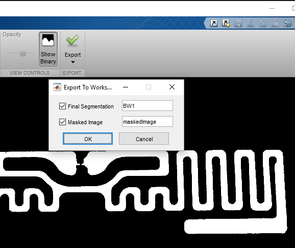
Export Code and Boundary
The color based segmentation process yields the mask of the antenna image. Use the export option on the app, to obtain a function and the boundary information which can then be used in a script for further processing (such as this one).
Boundary Clean-up
Read Image, Create Mask and Visualize
The image of the RFID tag is imported into the workspace and the boundary is generated by using the exported code from the Image Segmenter app.
I = imread("IMG_2151.JPG");
BWf = createMask_2151(I);
figure
imshow(BWf)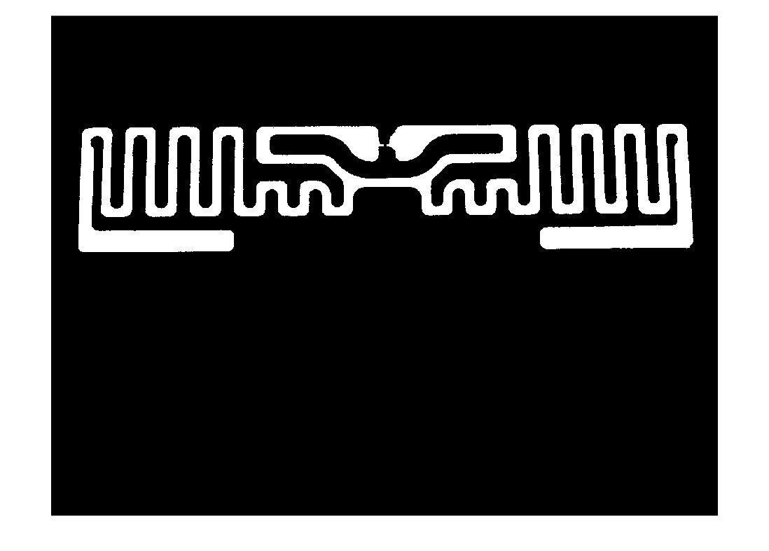
Calculate Boundaries in Cartesian Space
For performing full-wave analysis on this structure the next step is to convert the pixel space representation of the boundary to a Cartesian space representation. To do this, extract the maximum and minimum pixel indices in the x, y dimensions and scale it based on overall tag dimensions in terms of its length and width.
B = bwboundaries(BWf);
xmax = max(B{1}(:,1));
xmin = min(B{1}(:,1));
ymax = max(B{1}(:,2));
ymin = min(B{1}(:,2));

% Scale per pixel based on tag dimensions
L = 18.61e-3;
W = 72.27e-3;
LperColpixel = L/(xmax-xmin);
WperRowpixel = W/(ymax-ymin);
Bp = B;
for i = 1:length(Bp)
    Bp{i} = [Bp{i}(:,1).*LperColpixel Bp{i}(:,2).*WperRowpixel zeros(size(Bp{i},1),1)];
end
p = cell2mat(Bp);
x = p(:,1);
y = p(:,2);
figure
plot(x,y,'*')
grid on
axis equal
xlabel("x (m)")
ylabel("y (m)")
title("Boundary points")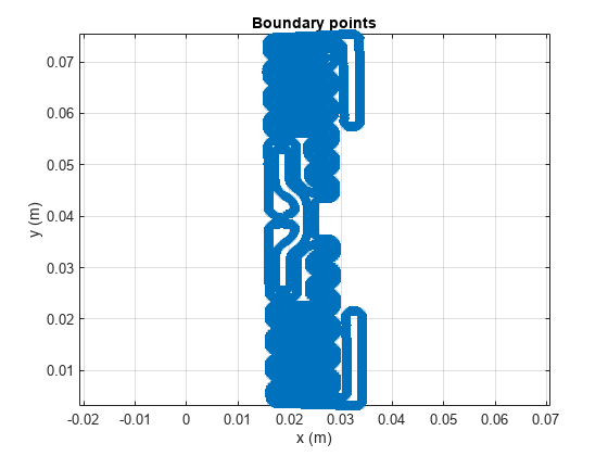
Reduce Boundary Points
The boundary has 28000 points, and this results in a very large mesh size. Downsample this boundary by a factor of 39. The downsample factor is chosen such that it still represents the boundary details accurately based on a simple visual inspection.
D = 39;
xD = x(1:D:end);
yD = y(1:D:end);
BpD{1} = Bp{1}(1:D:end,:);
figure
hold on
plot(xD,yD,'r*')
shg
grid on
axis equal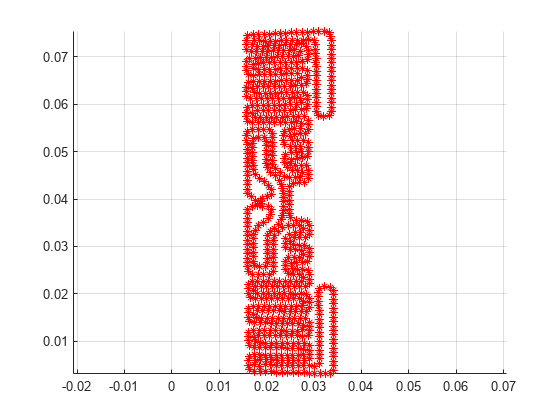
Create Layer for PCB Stack
Create a shape from the boundary.
pol = antenna.Polygon(Vertices=BpD{1});Create antenna feed
The feed region of the tag still has some sharp artifacts in the boundary. This must be cleaned up prior to defining the feed. Use a boolean subtract operation by creating a rectangle to remove this artifact.
rect1 = antenna.Rectangle(Length=5e-3, Width=2e-3,...
    Center=[0.019 0.0392]);
The final step, is to define the feeding strip. Add a feed in the form of a rectangle.
rect2 = antenna.Rectangle(Length=0.25e-3, Width=2e-3,...
    Center=[0.0185 0.0392]);
Perform addition and subtraction operations on these shapes to create the resultant shape.
final_shape = pol - rect1 + rect2;
Create PCB Stack
Assign the resultant shape generated as the layer for PCB stack. Specify the FeedLocation property appropriately so that it lies on this layer.
p = pcbStack;
p.Layers = {final_shape};
p.BoardShape = antenna.Rectangle(Length=1,Width=1);
p.FeedLocations = [0.0185 0.0392 1];
p.FeedDiameter = 1.25e-4;
figure
title("PCB Stack Antenna Element")
show(p)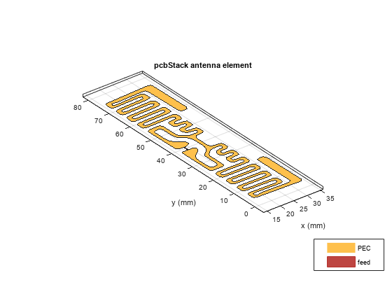
Port Analysis - Impedance Behavior vs. Frequency
Determine the port characteristics of this antenna by executing an impedance analysis over a coarse sampled frequency range. The tag is expected to operate in the UHF band, between 800 - 900 MHz. The frequency range extends slightly past 900 MHz.
f_coarse = linspace(0.8e9,0.95e9,21);
figure
impedance(p,f_coarse)
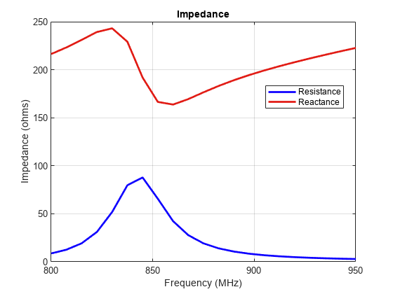
Tune Tag for Resonance
The tag is inductive and has a good Resistive component at approximately 854 MHz. Moreover the reactance shows the classic parallel resonance curve around that frequency. Typically, the input impedance of the chip would be complex, to match to the tag. Use Load property on the antenna to cancel the inductive component. Since the reactance is about 200 create a load with reactance of -200 and add it to the antenna model.
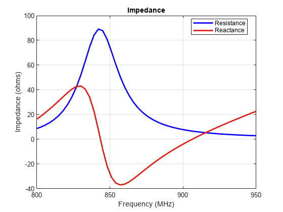
X = -1i*200;
zl = lumpedElement;
zl.Impedance = X;
p.Load = zl;
Recalculate impedance with the load in place at the feed, the inductive part of the reactance must be canceled at 854 MHz. Confirm this by analyzing the impedance over a fine frequency range. The reactance at 854 MHz should be approximately 0 ohms.
f_fine = linspace(0.8e9,0.95e9,51);
figure
impedance(p,f_fine)
Surface Analysis - Current behavior at Center Frequency
At the center frequency visualize the current distribution on the antenna surface.
figure
current(p,854e6,Scale="log10");
view(0,90);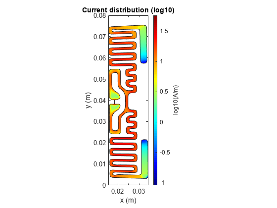
Field Analysis - Pattern at Center Frequency
RFID tags typically have an Omnidirectional far-field pattern in one plane. Visualize the far-field radiation pattern of the tag.
figure
pattern(p,854e6)
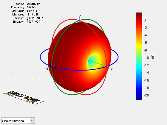
The tag has a gain of approximately 2 dBi at 854 MHz.
Conclusion
A procedure for identifying the antenna boundary from a photograph, conversion into a geometric model of the antenna and its subsequent full-wave analysis has been detailed in this example. These steps are graphically depicted as shown:
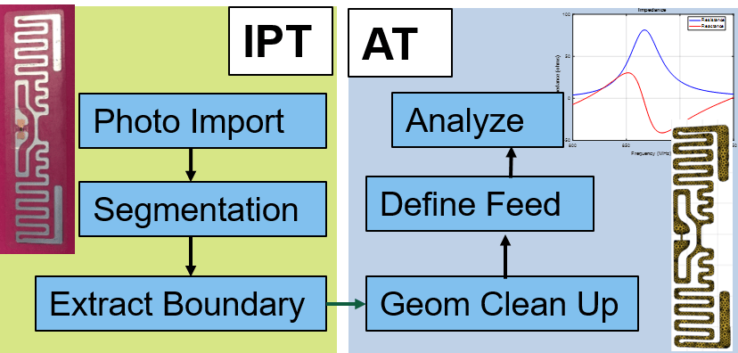
The antenna performance characteristics obtained from this procedure are good enough for further integration into a larger system simulation.