cepstralCoefficients
Extract cepstral coefficients
Description
coeffs = cepstralCoefficients(S,Name=Value)
For example, coeffs =
cepstralCoefficients(S,Rectification="cubic-root") uses cubic-root rectification
to calculate the coefficients.
Examples
Read an audio file into the workspace.
[audioIn,fs] = audioread('SpeechDFT-16-8-mono-5secs.wav');Convert the audio signal to a frequency-domain representation using 30 ms windows with 15 ms overlap. Because the input is real and therefore the spectrum is symmetric, you can use just one side of the frequency domain representation without any loss of information. Convert the complex spectrum to the magnitude spectrum: phase information is discarded when calculating mel frequency cepstral coefficients (MFCC).
windowLength = round(0.03*fs);
overlapLength = round(0.015*fs);
S = stft(audioIn,"Window",hann(windowLength,"periodic"),"OverlapLength",overlapLength,"FrequencyRange","onesided");
S = abs(S);
Design a one-sided frequency-domain mel filter bank. Apply the filter bank to the frequency-domain representation to create a mel spectrogram.
filterBank = designAuditoryFilterBank(fs,'FFTLength',windowLength);
melSpec = filterBank*S;
Call cepstralCofficients with the mel spectrogram to create MFCC.
melcc = cepstralCoefficients(melSpec);
Read an audio signal and convert it to a one-sided magnitude short-time Fourier transform. Use a 50 ms periodic Hamming window with a 10 ms hop.
[audioIn,fs] = audioread('NoisySpeech-16-22p5-mono-5secs.wav');

windowLength = round(0.05*fs);
hopLength = round(0.01*fs);
overlapLength = windowLength - hopLength;

S = stft(audioIn,"Window",hamming(windowLength,'periodic'),"OverlapLength",overlapLength,"FrequencyRange","onesided");
S = abs(S);
Design a one-sided frequency-domain gammatone filter bank. Apply the filter bank to the frequency-domain representation to create a gammatone spectrogram.
filterBank = designAuditoryFilterBank(fs,'FFTLength',windowLength,"FrequencyScale","erb");
gammaSpec = filterBank*S;
Call cepstralCoefficients with the gammatone spectrogram to create gammatone frequency cepstral coefficients. Use a cubic-root rectification.
gammacc = cepstralCoefficients(gammaSpec,"Rectification","cubic-root");
Cepstral coefficients are commonly used as compact representations of audio signals. Generally, they are calculated after an audio signal is passed through a filter bank and the energy in the individual filters is summed. Researchers have proposed various filter banks based on psychoacoustic experiments (such as mel, Bark, and ERB). Using the cepstralCoefficients function, you can define your own custom filter bank and then analyze the resulting cepstral coefficients.
Read in an audio file for analysis.
[audioIn,fs] = audioread('Counting-16-44p1-mono-15secs.wav');Design a filter bank that consists of 20 triangular filters with band edges over the range 62.5 Hz to 8000 Hz. Spread the filters evenly in the log domain. For simplicity, design the filters in bins. Most popular auditory filter banks are designed in a continuous domain, such as Hz, mel, or Bark, and then warped back to bins.
numFilters =20; filterbankStart =
62.5; filterbankEnd =
8000; numBandEdges = numFilters + 2; NFFT = 1024; filterBank = zeros(numFilters,NFFT); bandEdges = logspace(log10(filterbankStart),log10(filterbankEnd),numBandEdges); bandEdgesBins = round((bandEdges/fs)*NFFT) + 1; for ii = 1:numFilters filt = triang(bandEdgesBins(ii+2)-bandEdgesBins(ii)); leftPad = bandEdgesBins(ii); rightPad = NFFT - numel(filt) - leftPad; filterBank(ii,:) = [zeros(1,leftPad),filt',zeros(1,rightPad)]; end
Plot the filter bank.
frequencyVector = (fs/NFFT)*(0:NFFT-1);
plot(frequencyVector,filterBank');
xlabel('Hz')
axis([0 frequencyVector(NFFT/2) 0 1])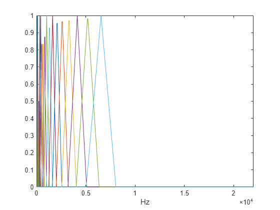
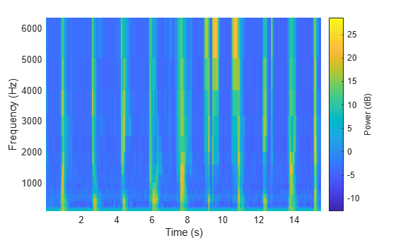
Transform the audio signal using the stft function, and then apply the custom filter bank. Apply the filter bank to the frequency-domain representation to create a custom auditory spectrogram. Plot the spectrogram.
[S,~,t] = stft(audioIn,fs,"Window",hann(NFFT,'periodic'),"FrequencyRange","twosided");
S = abs(S);
spec = filterBank*S;

surf(t,bandEdges(2:end-1),10*log10(spec),'EdgeColor','none')
view([0,90])
axis([t(1) t(end) bandEdges(2) bandEdges(end-1)])
xlabel('Time (s)')
ylabel('Frequency (Hz)')
c = colorbar;
c.Label.String = 'Power (dB)';
Call cepstralCoefficients with the custom auditory spectrogram to create custom cepstral coefficients.
ccc = cepstralCoefficients(S);
Create a dsp.AudioFileReader object to read in audio frame-by-frame. Create a dsp.AsyncBuffer object to buffer the input into overlapped frames.
fileReader = dsp.AudioFileReader("Ambiance-16-44p1-mono-12secs.wav");
buff = dsp.AsyncBuffer;
Design a two-sided mel filter bank that is compatible with 30 ms windows.
windowLength = round(0.03*fileReader.SampleRate);
filterBank = designAuditoryFilterBank(fileReader.SampleRate,"FFTLength",windowLength,"OneSided",false);
In an audio stream loop:
Read a frame of data from the audio file.
Write the frame of data to the buffer.
If enough data is available for a hop, read a 30 ms frame of data from the buffer with a 20 ms overlap between frames.
Transform the data to a magnitude spectrum.
Apply the mel filter bank to create a mel spectrum.
Call
cepstralCoefficientsto return the mel frequency cepstral coefficients (MFCC).
win = hann(windowLength,'periodic');
overlapLength = round(0.02*fileReader.SampleRate);
hopLength = windowLength - overlapLength;

while ~isDone(fileReader)
    audioIn = fileReader();
    write(buff,audioIn);
    while buff.NumUnreadSamples > hopLength
        x = read(buff,windowLength,overlapLength);
        X = abs(fft(x.*win));
        melSpectrum = filterBank*X;
        melcc = cepstralCoefficients(melSpectrum);
    end
end
Input Arguments
Name-Value Arguments
Output Arguments
Algorithms
Given an auditory spectrogram, the algorithm to extract N cepstral coefficients from each individual spectrum comprises the following steps.
Rectify the spectrum by applying a logarithm, cubic root, or optionally perform no rectification.
Apply the discrete cosine transform (DCT-II) to the rectified spectrum.
Return the first N coefficients from the cepstral representation.
For more information, see [1].
References
[1] Rabiner, Lawrence R., and Ronald W. Schafer. Theory and Applications of Digital Speech Processing. Upper Saddle River, NJ: Pearson, 2010.
Extended Capabilities
Version History
Introduced in R2020b
See Also
Functions
mfcc|gtcc|audioDelta|designAuditoryFilterBank|melSpectrogram|stft