interface
Syntax
Description
specifies physical couplings between components sysCon
= interface(sys
,C1,IC1,C2,IC2)C1
and
C2
in the second-order sparse model sys
.
IC1
and IC2
contain the indices of the coupled
degrees of freedom (DOFs) relative to the DOFs of C1
and
C2
. The physical interface is assumed rigid and satisfies the standard
consistency and equilibrium conditions. sysCon
is the resultant model
with the specified physical connections. Use showStateInfo
to get the list of all available components of sys
.
specifies the assembly method. By default, sysCon
= interface(___,method
)method
=
'dual'
and the function uses the dual-assembly method of physical
coupling. Set method
= 'primal'
to use the
primal-assembly method of physical coupling. For more information, see Algorithms.
Examples
Physical Connections Between Components in Sparse Second-Order Model
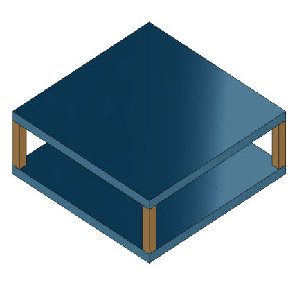
For this example, consider a structural model that consists of two square plates connected with pillars at each vertex as depicted in the figure below. The lower plate is attached rigidly to the ground while the pillars are attached rigidly to each vertex of the square plate.
Load the finite element model matrices contained in platePillarModel.mat
and create the sparse second-order model representing the above system.
load('platePillarModel.mat') model = ... mechss(M1,[],K1,B1,F1,'Name','Plate1') + ... mechss(M2,[],K2,B2,F2,'Name','Plate2') + ... mechss(Mp,[],Kp,Bp,Fp,'Name','Pillar3') + ... mechss(Mp,[],Kp,Bp,Fp,'Name','Pillar4') + ... mechss(Mp,[],Kp,Bp,Fp,'Name','Pillar5') + ... mechss(Mp,[],Kp,Bp,Fp,'Name','Pillar6'); sys = model;
Use showStateInfo
to examine the components of the mechss
model object.
showStateInfo(sys)
The state groups are: Type Name Size ---------------------------- Component Plate1 2646 Component Plate2 2646 Component Pillar3 132 Component Pillar4 132 Component Pillar5 132 Component Pillar6 132
Now, load the interfaced degree of freedom (DOF) index data from dofData.mat
and use interface
to create the physical connections between the two plates and the four pillars. dofs
is a 6x7
cell array where the first two rows contain DOF index data for the first and second plates while the remaining four rows contain index data for the four pillars. By default, the function uses dual-assembly method of physical coupling.
load('dofData.mat','dofs') for i=3:6 sys = interface(sys,"Plate1",dofs{1,i},"Pillar"+i,dofs{i,1}); sys = interface(sys,"Plate2",dofs{2,i},"Pillar"+i,dofs{i,2}); end
Specify connection between the bottom plate and the ground.
sysConDual = interface(sys,"Plate2",dofs{2,7});
Use showStateInfo
to confirm the physical interfaces.
showStateInfo(sysConDual)
The state groups are: Type Name Size ----------------------------------- Component Plate1 2646 Component Plate2 2646 Component Pillar3 132 Component Pillar4 132 Component Pillar5 132 Component Pillar6 132 Interface Plate1-Pillar3 12 Interface Plate2-Pillar3 12 Interface Plate1-Pillar4 12 Interface Plate2-Pillar4 12 Interface Plate1-Pillar5 12 Interface Plate2-Pillar5 12 Interface Plate1-Pillar6 12 Interface Plate2-Pillar6 12 Interface Plate2-Ground 6
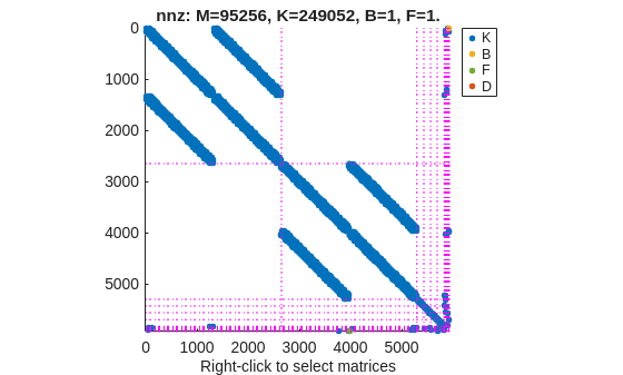
You can use spy
to visualize the sparse matrices in the final model.
spy(sysConDual)
Now, specify physical connections using the primal-assembly method.
sys = model; for i=3:6 sys = interface(sys,"Plate1",dofs{1,i},"Pillar"+i,dofs{i,1},'primal'); sys = interface(sys,"Plate2",dofs{2,i},"Pillar"+i,dofs{i,2},'primal'); end sysConPrimal = interface(sys,"Plate2",dofs{2,7},'primal');
Use showStateInfo
to confirm the physical interfaces.
showStateInfo(sysConPrimal)
The state groups are: Type Name Size ---------------------------- Component Plate1 2646 Component Plate2 2640 Component Pillar3 108 Component Pillar4 108 Component Pillar5 108 Component Pillar6 108
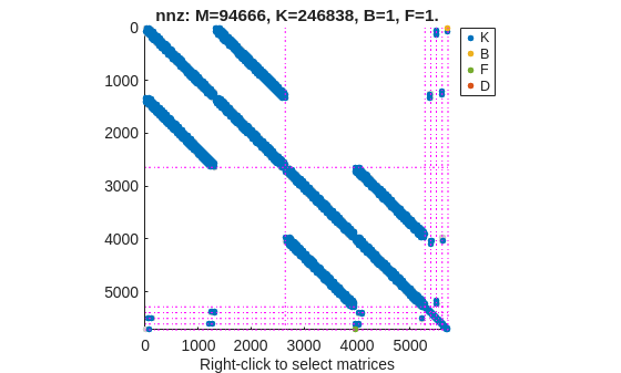
Primal assembly eliminates half of the redundant DOFs associated with the shared set of DOFs in the global finite element mesh.
You can use spy
to visualize the sparse matrices in the final model.
spy(sysConPrimal)
The data set for this example was provided by Victor Dolk from ASML.
Input Arguments
sys
— Sparse second-order model
mechss
model object
Sparse second-order model, specified as a mechss
model object.
For more information, see mechss
.
C
— Components to connect
string | array of character vectors
Components of sys
to connect, specified as a string or an array
of character vectors. Use showStateInfo
to get the list of all available components of
sys
.
IC
— Index information of components to connect
Nc
-by-Ni
cell array
Index information of components to connect, specified as an
Nc
-by-Ni
cell array, where Nc
is the number of components and Ni
is the number of physical
interfaces.
KI
— Stiffness matrix
Nq
-by-Nq
sparse matrix
Stiffness matrix, specified as an Nq
-by-Nq
sparse matrix, where Nq
is the number of DOFs in
sys
.
CI
— Damping matrix
Nq
-by-Nq
sparse matrix
Damping matrix, specified as an Nq
-by-Nq
sparse matrix, where Nq
is the number of DOFs in
sys
.
method
— Assembly method
'dual'
(default) | 'primal'
Interface assembly method, specified as one of the following:
'dual'
— Use the dual-assembly method of physical coupling. This method maintains sparsity at the expense of additional algebraic variables.'primal'
— Use the primal-assembly method of physical coupling. This method uses a minimal number of DOFs but the system may suffer from fill-in.
For more information, see Algorithms.
Output Arguments
sysCon
— Output system with physical interfaces
mechss
model object
Output system with physical interfaces, returned as a mechss
model object. Use showStateInfo
to examine the list of physical interfaces in the
system.
Algorithms
Rigid Interface
For n substructures in the physical domain, the sparse matrices in block diagonal form are:
Two interfaced components share a set of DOFs in the global finite element mesh q: the subset N1 of DOFs from the first component coincides with the subset N2 of DOFs from the second component. The coupling between the two components is rigid only if:
The displacements q at the shared DOFs are the same for both components.
The forces g one component exerts on the other are opposite (by the action/reaction principle).
These relations can be summarized as:
where H is a localisation matrix with entries 0, 1, or –1. The equation Hq = 0 is equivalent to q(N1) = q(N2), and the equation g = −HT λ is equivalent to g(N1) = −λ and g(N2) = λ.
The equations
can be combined in the differential-algebraic equation (DAE) form:
This DAE model is called the dual-assembly model of the overall structure. While the principle was explained for two components, this model can accommodate multiple interfaces, including interfaces involving more than two components.
For rigid interfaces, primal assembly consists of eliminating half of the redundant DOFs associated with the following constraint.
If Hq = 0 is the matrix expression of this constraint, this amounts to writing q = Lqr. Here, qr is the set of independent (free) DOFs and L spans the null space of H.
Using q = Lqr, the equations
become
Using LTHT = (HL)T = 0, the first part of equation can be projected onto the range of L by premultiplying by LT:
This is the primal-assembly model of the overall structure. It has 2N1 fewer algebraic variables than its dual-assembly counterpart, at the expense of potential fill-in in the reduced M, C, and K.
Nonrigid Interface
In non-rigid interfaces, the displacements q1(N1) and q2(N2) are allowed to differ and the internal force is given by:
This models spring-damper-like connections between DOFs N1 in the first component and DOFs N2 in the second component. Going from rigid to non-rigid connection eliminates the algebraic constraints Hq = 0 and explicates the internal forces. Then, eliminate λ to obtain:
This is the set of the primal-assembly equations for non-rigid coupling form that remains symmetric when the uncoupled model is symmetric. A drawback of this form is that the coupling terms and may cause fill-in. To avoid this, you can use the equivalent dual-assembly form:
Version History
Introduced in R2020b
Ouvrir l'exemple
Vous possédez une version modifiée de cet exemple. Souhaitez-vous ouvrir cet exemple avec vos modifications ?
Commande MATLAB
Vous avez cliqué sur un lien qui correspond à cette commande MATLAB :
Pour exécuter la commande, saisissez-la dans la fenêtre de commande de MATLAB. Les navigateurs web ne supportent pas les commandes MATLAB.
Select a Web Site
Choose a web site to get translated content where available and see local events and offers. Based on your location, we recommend that you select: .
You can also select a web site from the following list:
How to Get Best Site Performance
Select the China site (in Chinese or English) for best site performance. Other MathWorks country sites are not optimized for visits from your location.
Americas
- América Latina (Español)
- Canada (English)
- United States (English)
Europe
- Belgium (English)
- Denmark (English)
- Deutschland (Deutsch)
- España (Español)
- Finland (English)
- France (Français)
- Ireland (English)
- Italia (Italiano)
- Luxembourg (English)
- Netherlands (English)
- Norway (English)
- Österreich (Deutsch)
- Portugal (English)
- Sweden (English)
- Switzerland
- United Kingdom (English)