Convert Discrete-Time System to Continuous Time
This example shows how to convert a discrete-time system to continuous time using d2c, and compare the results using two different interpolation methods.
Convert the following second-order discrete-time system to continuous time using the zero-order hold (ZOH) method:
G = zpk(-0.5,[-2,5],1,0.1);
Gcz = d2c(G)
Warning: The model order was increased to handle real negative poles.
Gcz =

   2.6663 (s^2 + 14.28s + 780.9)
  -------------------------------
  (s-16.09) (s^2 - 13.86s + 1035)

Continuous-time zero/pole/gain model.
Model Properties
When you call d2c without specifying a method, the function uses ZOH by default. The ZOH interpolation method increases the model order for systems that have real negative poles. This order increase occurs because the interpolation algorithm maps real negative poles in the domain to pairs of complex conjugate poles in the domain.
Convert G to continuous time using the Tustin method.
Gct = d2c(G,'tustin')Gct =
0.083333 (s+60) (s-20)
----------------------
(s-60) (s-13.33)
Continuous-time zero/pole/gain model.
Model Properties
In this case, there is no order increase.
Compare frequency responses of the interpolated systems with that of G.
bode(G,Gcz,Gct)
legend('G','Gcz','Gct')
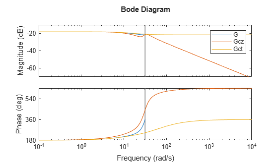
In this case, the Tustin method provides a better frequency-domain match between the discrete system and the interpolation. However, the Tustin interpolation method is undefined for systems with poles at z = -1 (integrators), and is ill-conditioned for systems with poles near z = 1.