Create 360° Bird's-Eye-View Image Around a Vehicle
This example shows how to create a 360° bird's-eye-view image around a vehicle for use in a surround view monitoring system. It then shows how to generate code for the same bird's-eye-view image creation algorithm and verify the results.
Overview
Surround view monitoring is an important safety feature provided by advanced driver-assistance systems (ADAS). These monitoring systems reduce blind spots and help drivers understand the relative position of their vehicle with respect to the surroundings, making tight parking maneuvers easier and safer. A typical surround view monitoring system consists of four fisheye cameras, with a 180° field of view, mounted on the four sides of the vehicle. A display in the vehicle shows the driver the front, left, right, rear, and bird's-eye view of the vehicle. While the four views from the four cameras are trivial to display, creating a bird's-eye view of the vehicle surroundings requires intrinsic and extrinsic camera calibration and image stitching to combine the multiple camera views.
In this example, you first calibrate the multi-camera system to estimate the camera parameters. You then use the calibrated cameras to create a bird's-eye-view image of the surroundings by stitching together images from multiple cameras.
Calibrate the Multi-Camera System
First, calibrate the multi-camera system by estimating the camera intrinsic and extrinsic parameters by constructing a monoCamera object for each camera in the multi-camera system. For illustration purposes, this example uses images taken from eight directions by a single camera with a 78˚ field of view, covering 360˚ around the vehicle. The setup mimics a multi-camera system mounted on the roof of a vehicle.
Estimate Monocular Camera Intrinsics
Camera calibration is an essential step in the process of generating a bird's-eye view. It estimates the camera intrinsic parameters, which are required for estimating camera extrinsics, removing distortion in images, measuring real-world distances, and finally generating the bird's-eye-view image.
In this example, the camera was calibrated using a checkerboard calibration pattern in the Using the Single Camera Calibrator App and the camera parameters were exported to cameraParams.mat. Load these estimated camera intrinsic parameters.
ld = load("cameraParams.mat");Since this example mimics eight cameras, copy the loaded intrinsics eight times. If you are using eight different cameras, calibrate each camera separately and store their intrinsic parameters in a cell array named intrinsics.
numCameras = 8;
intrinsics = cell(numCameras, 1);

intrinsics(:) = {ld.cameraParams.Intrinsics};
Estimate Monocular Camera Extrinsics
In this step, you estimate the extrinsics of each camera to define its position in the vehicle coordinate system. Estimating the extrinsics involves capturing the calibration pattern from the eight cameras in a specific orientation with respect to the road and the vehicle. In this example, you use the horizontal orientation of the calibration pattern. For details on the camera extrinsics estimation process and pattern orientation, see Calibrate a Monocular Camera.
Place the calibration pattern in the horizontal orientation parallel to the ground, and at an appropriate height such that all the corner points of the pattern are visible. Measure the height after placing the calibration pattern and the size of a square in the checkerboard. In this example, the pattern was placed horizontally at a height of 62.5 cm to make the pattern visible to the camera. The size of a square in the checkerboard pattern was measured to be 29 mm.
% Measurements in meters
patternOriginHeight = 0.625; % meter
squareSize = 0.029; % meter
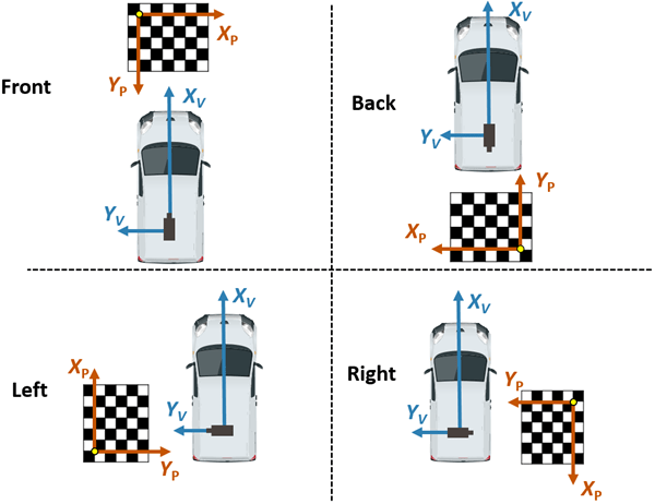
The following figure illustrates the proper orientation of the calibration pattern for cameras along the four principal directions, with respect to the vehicle axes. However, for generating the bird's-eye view, this example uses four additional cameras oriented along directions that are different from the principal directions. To estimate extrinsics for those cameras, choose and assign the preferred orientation among the four principal directions. For example, if you are capturing from a front-facing camera, align the X- and Y- axes of the pattern as shown in the following figure.
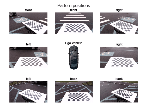
The variable patternPositions stores the preferred orientation choices for all the eight cameras. These choices define the relative orientation between the pattern axes and the vehicle axes for estimateMonoCameraParameters function. Display the images arranged by their camera positions relative to the vehicle.
patternPositions = ["front", "left" , "left" , "back" ,...
                    "back" , "right", "right", "front"];
extrinsicsCalibrationImages = cell(1, numCameras);
for i = 1:numCameras
    filename = "extrinsicsCalibrationImages/extrinsicsCalibrationImage" +  string(i) + ".jpg";
    extrinsicsCalibrationImages{i} = imread(filename);
end
helperVisualizeScene(extrinsicsCalibrationImages, patternPositions)
To estimate the extrinsic parameters of one monocular camera, follow these steps:
Remove distortion in the image.
Detect the corners of the checkerboard square in the image.
Generate the world points of the checkerboard.
Use
estimateMonoCameraParametersfunction to estimate the extrinsic parameters.Use the extrinsic parameters to create a
monoCameraobject, assuming that the location of the sensor location at vehicle coordinate system's origin.
In this example, the setup uses a single camera that was rotated manually around a camera stand. Although the camera's focal center had moved during this motion, for simplicity, this example assumes that the sensor remained at the same location (at origin). However, distances between cameras on a real vehicle can be measured and entered in the sensor location property of monoCamera.
monoCams = cell(1, numCameras);
for i = 1:numCameras
    % Undistort the image.
    [undistortedImage, newIntrinsics] = undistortImage(extrinsicsCalibrationImages{i}, intrinsics{i});

    % Detect checkerboard points.
    [imagePoints, patternDims] = detectCheckerboardPoints(undistortedImage, PartialDetections=false);

    % Generate world points of the checkerboard.
    worldPoints = patternWorldPoints("checkerboard", patternDims, squareSize);

    % Estimate extrinsic parameters of the monocular camera.
    [pitch, yaw, roll, height] = estimateMonoCameraParameters(newIntrinsics, ...
                                     imagePoints, worldPoints, patternOriginHeight,...
                                     PatternPosition=patternPositions(i));

    % Create a monoCamera object, assuming the camera is at origin.
    monoCams{i} = monoCamera(newIntrinsics, height, ...
                             Pitch=pitch, ...
                             Yaw=yaw, ...
                             Roll=roll, ...
                             SensorLocation=[0, 0]);
end
Create 360**°** Bird's-Eye-View Image
Use the monoCamera objects configured using the estimated camera parameters to generate individual bird's-eye-view images from the eight cameras. Stitch them to create the 360**°** bird's-eye-view image.
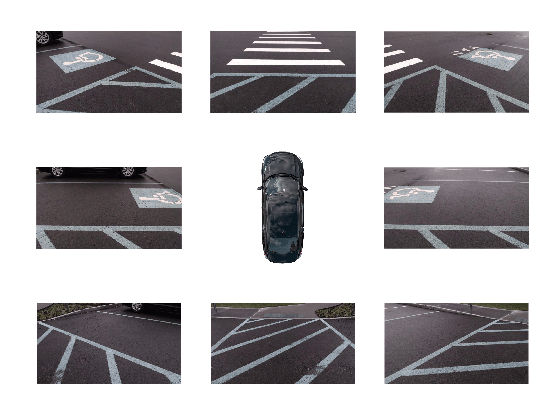
Capture the scene from the cameras and load the images in the MATLAB workspace.
sceneImages = cell(1, numCameras);
for i = 1:numCameras
    filename = "sceneImages/sceneImage" + string(i) + ".jpg";
    sceneImages{i} = imread(filename);
end
helperVisualizeScene(sceneImages)
Transform Images to Bird's-Eye View
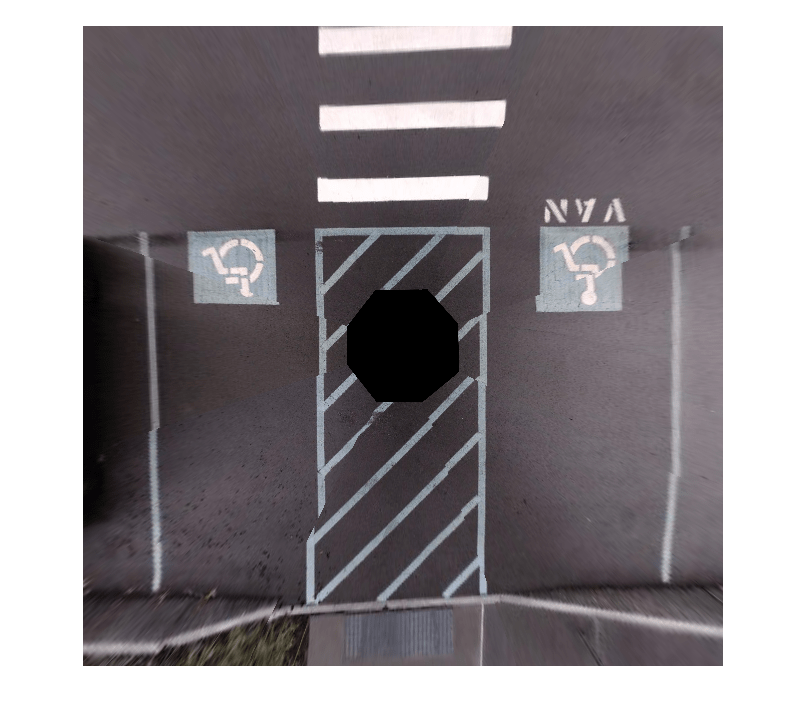
Specify the rectangular area around the vehicle that you want to transform into a bird's-eye view and the output image size. In this example, the farthest objects in captured images are about 4.5 m away.
Create a square output view that covers 4.5 m radius around the vehicle.
distFromVehicle = 4.5; % in meters
outView = [-distFromVehicle, distFromVehicle, ... % [xmin, xmax,
           -distFromVehicle, distFromVehicle];    %  ymin, ymax]
outImageSize = [640, NaN];
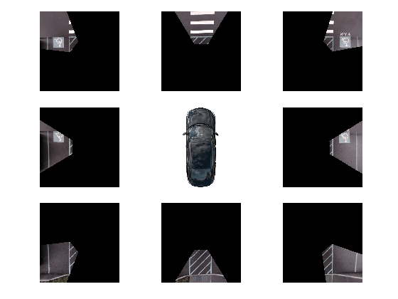
To create the bird's-eye-view image from each monoCamera object, follow these steps.
Remove distortion in the image.
Create a
birdsEyeViewobject.Transform the undistorted image to a bird's-eye-view image using the
transformImagefunction.
bevImgs = cell(1, numCameras);
birdsEye = cell(1, numCameras);
for i = 1:numCameras
    undistortedImage = undistortImage(sceneImages{i}, intrinsics{i});
    birdsEye{i} = birdsEyeView(monoCams{i}, outView, outImageSize);
    bevImgs{i}  = transformImage(birdsEye{i}, undistortedImage);
end
helperVisualizeScene(bevImgs)
Test the accuracy of the extrinsics estimation process by using the helperBlendImages function which blends the eight bird's-eye-view images. Then display the image.
tiled360DegreesBirdsEyeView = zeros(640, 640, 3);
for i = 1:numCameras
    tiled360DegreesBirdsEyeView = helperBlendImages(tiled360DegreesBirdsEyeView, bevImgs{i});
end
figure
imshow(tiled360DegreesBirdsEyeView)
For this example, the initial results from the extrinsics estimation process contain some misalignment. However, those can be attributed to the wrong assumption that the camera was located at the origin of the vehicle coordinate system. Correcting the misalignment requires image registration.
Register and Stitch Bird's-Eye-View Images
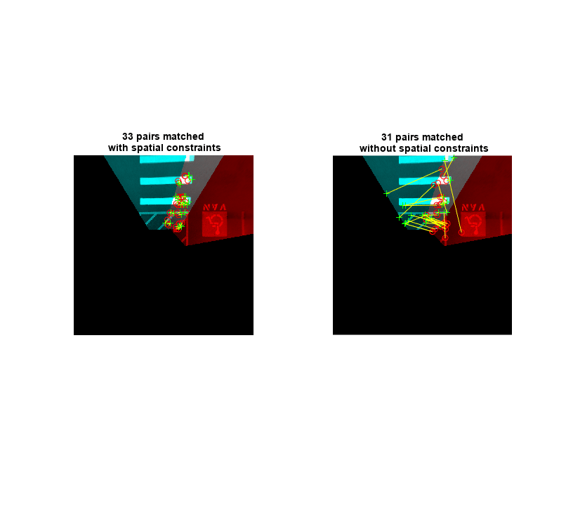
First, match the features. Compare and visualize the results of using matchFeatures with matchFeaturesInRadius, which enables you to restrict the search boundary using geometric constraints. Constrained feature matching can improve results when patterns are repetitive, such as on roads, where pavement markings and road signs are standard. In factory settings, you can design a more elaborate configuration of the calibration patterns and textured background that further improves the calibration and registration process. The Create Panorama example explains in detail how to register multiple images and stitch them to create a panorama. The results show that constrained feature matching using matchFeaturesInRadius matches only the corresponding feature pairs in the two images and discards any features corresponding to unrelated repetitive patterns.
% The last two images of the scene best demonstrate the advantage of
% constrained feature matching as they have many repetitive pavement
% markings.
I = bevImgs{7};
J = bevImgs{8};

% Extract features from the two images.
grayImage = rgb2gray(I);
pointsPrev = detectKAZEFeatures(grayImage);
[featuresPrev, pointsPrev] = extractFeatures(grayImage, pointsPrev);

grayImage = rgb2gray(J);
points = detectKAZEFeatures(grayImage);
[features, points] = extractFeatures(grayImage, points);

% Match features using the two methods.
indexPairs1 = matchFeaturesInRadius(featuresPrev, features, points.Location, ...
                                   pointsPrev.Location, 15, ...
                                   MatchThreshold=10, MaxRatio=0.6);

indexPairs2 = matchFeatures(featuresPrev, features, MatchThreshold=10, ...
                            MaxRatio=0.6);

% Visualize the matched features.
tiledlayout(1,2)
nexttile
showMatchedFeatures(I, J, pointsPrev(indexPairs1(:,1)), points(indexPairs1(:,2)))
title(sprintf('%d pairs matched\n with spatial constraints', size(indexPairs1, 1)))

nexttile
showMatchedFeatures(I, J, pointsPrev(indexPairs2(:,1)), points(indexPairs2(:,2)))
title(sprintf('%d pairs matched\n without spatial constraints', size(indexPairs2,1)))
The functions helperRegisterImages and helperStitchImages have been written based on the Create Panorama example using matchFeaturesInRadius. Note that traditional panoramic stitching is not enough for this application as each image is registered with respect to the previous image alone. Consequently, the last image might not align accurately with the first image, resulting in a poorly aligned 360° surround view image.
This drawback in the registration process can be overcome by registering the images in batches:
Register and stitch the first four images to generate the image of left side of the vehicle.
Register and stitch the last four images to generate the image of right side of the vehicle.
Register and stitch the left side and right side to get the complete 360° of the bird's-eye-view image of the scene.
Note the use of larger matching radius for stitching images in step 3 compared to steps 1 and 2. This is because of the change in the relative positions of the images during the first two registration steps.
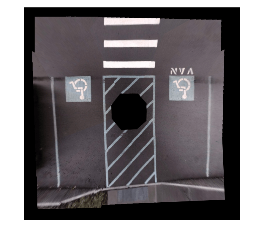
% Cell array holding two sets of transformations for left and right sides
finalTforms = cell(1,2);

% Combine the first four images to get the stitched leftSideview and the
% spatial reference object Rleft.
radius = 15;
leftImgs = bevImgs(1:4);
finalTforms{1} = helperRegisterImages(leftImgs, radius);
[leftSideView, Rleft] = helperStitchImages(leftImgs, finalTforms{1});

% Combine the last four images to get the stitched rightSideView.
rightImgs = bevImgs(5:8);
finalTforms{2} = helperRegisterImages(rightImgs, radius);
rightSideView = helperStitchImages(rightImgs, finalTforms{2});

% Combine the two side views to get the 360° bird's-eye-view in
% surroundView and the spatial reference object Rsurround
radius = 50;
imgs = {leftSideView, rightSideView};
tforms = helperRegisterImages(imgs, radius);
[surroundView, Rsurround] = helperStitchImages(imgs, tforms);
figure
imshow(surroundView)
Measure Distances in the 360° Bird's-Eye-View
One advantage in using bird's-eye-view images to measure distances is that the distances can be computed across the image owing to the planar nature of the ground. You can measure various distances that are useful for ADAS applications such as drawing proximity range guidelines and ego vehicle boundaries. Distance measurement involves transforming world points in the vehicle coordinate system to the bird's-eye-view image, which you can do using the vehicleToImage function. However, note that each of the eight bird's-eye-view images have undergone two geometric transformations during the image registration process. Thus, in addition to using the vehicleToImage function, you must apply these transformations to the image points. The helperVehicleToBirdsEyeView function applies these transformations. The points are projected to the first bird's-eye-view image, as this image has undergone the least number of transformations during the registration process.
Draw Proximity Range Guidelines
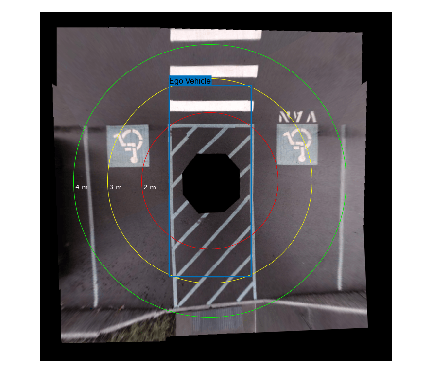
Circular parking range guidelines around the vehicle can assist drivers maneuvering in tight parking spots. Draw circular guidelines at 2, 3, and 4 meters on the 360° bird's-eye-view image:
Transform the vehicle center and a point in the circular guideline in the vehicle coordinate system, to the 360° bird's-eye-view image using
helperVehicleToBirdsEyeViewfunction.Calculate the radius of the circular guideline in pixels by finding the distance between the two transformed points.
Draw the guidelines using the
insertShapefunction and label the guidelines using theinsertTextfunction.
proximityRange = [2, 3, 4]; % in meters
colors         = ["red", "yellow", "green"];
refBirdsEye    = birdsEye{1};
Rout           = {Rleft, Rsurround};
vehicleCenter  = [0, 0];
vehicleCenterInImage = helperVehicleToBirdsEyeView(refBirdsEye, vehicleCenter, Rout);

for i = 1:length(proximityRange)

    % Estimate the radius of the circular guidelines in pixels given its
    % radius in meters.
    circlePoint         = [0, proximityRange(i)];
    circlePointInImage  = helperVehicleToBirdsEyeView(refBirdsEye, circlePoint, Rout);

    % Compute radius using euclidean norm.
    proximityRangeInPixels  = norm(circlePointInImage - vehicleCenterInImage, 2);

    surroundView = insertShape(surroundView, "Circle", [vehicleCenterInImage, proximityRangeInPixels], ...
                               LineWidth=1, ShapeColor=colors(i));

    labelText = string(proximityRange(i)) + " m";
    surroundView = insertText(surroundView, circlePointInImage, labelText,...
                              FontColor="White", ...
                              FontSize=14, ...
                              BoxOpacity=0);
end

imshow(surroundView)
Draw Ego Vehicle Boundary
Boundary lines for a vehicle help the driver understand the relative position of the vehicle with respect to the surroundings. Draw the ego vehicle's boundary using a similar procedure as that of drawing proximity guidelines. The helperGetVehicleBoundaryOnBEV function returns the corner points of the vehicle boundary on the 360° bird's-eye-view image given the vehicle position and size. Show the guidelines on the scene using the showShape function.
vehicleCenter = [0, 0];
vehicleSize   = [5.6, 2.4]; % length-by-width in meters
[polygonPoints, vehicleLength, vehicleWidth] = helperGetVehicleBoundaryOnBEV(refBirdsEye, ...
                                                                             vehicleCenter, ...
                                                                             vehicleSize, ...
                                                                             Rout);
showShape("polygon", polygonPoints, Label="Ego Vehicle")
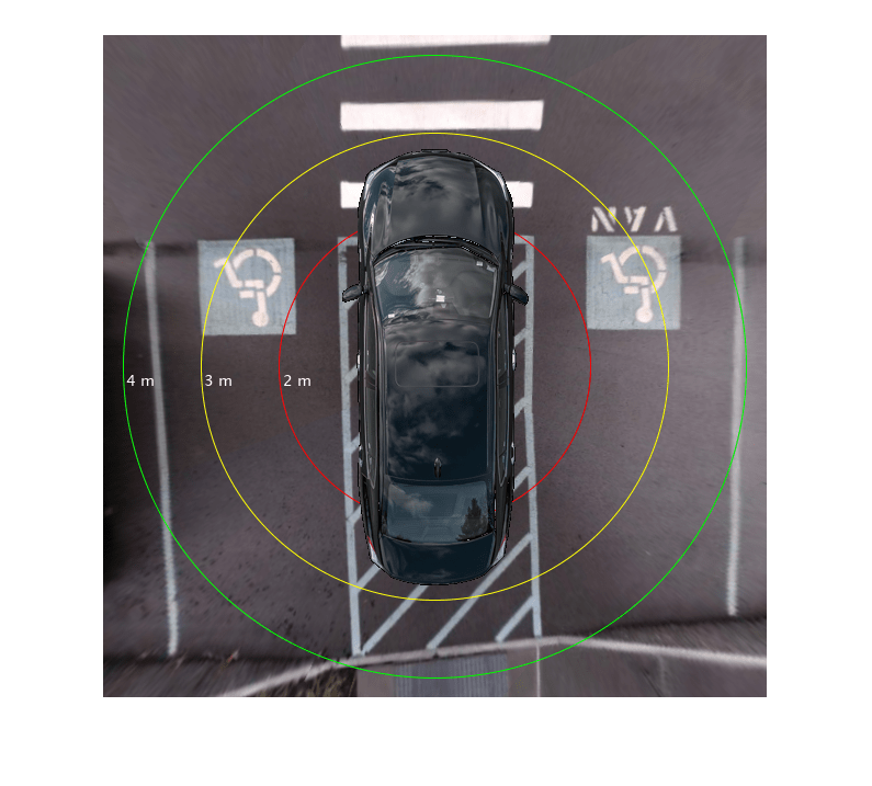
Additionally, you can also overlay a simulated vehicle on the scene for visually pleasing results.
% Read the picture of the simulation vehicle.
egoVehicleImage = imread("vehicle.png", BackgroundColor=[0 0 0]);

% Bring the simulation vehicle into the vehicle coordinate system.
egoVehicleImage = imresize(egoVehicleImage, [vehicleLength, vehicleWidth]);
vehicle    = zeros(size(surroundView), "uint8");
xIdx       = polygonPoints(1,1) + (1:vehicleWidth);
yIdx       = polygonPoints(1,2) + (1:vehicleLength);
vehicle(yIdx, xIdx, :) = egoVehicleImage;

% Overlay the simulation vehicle on the 360° bird's-eye-view image.
sceneBirdsEyeView = helperOverlayImage(vehicle, surroundView);
Finally, let's eliminate black borders in the image by selecting smaller range from the vehicle's coordinate system's origin.
distFromVehicle = 4.25; % in meters
[x, y, h, w] = helperGetImageBoundaryOnBEV(refBirdsEye, distFromVehicle, Rout);
croppedSceneBirdsEyeView = imcrop(sceneBirdsEyeView, [x, y, h, w]);
imshow(croppedSceneBirdsEyeView)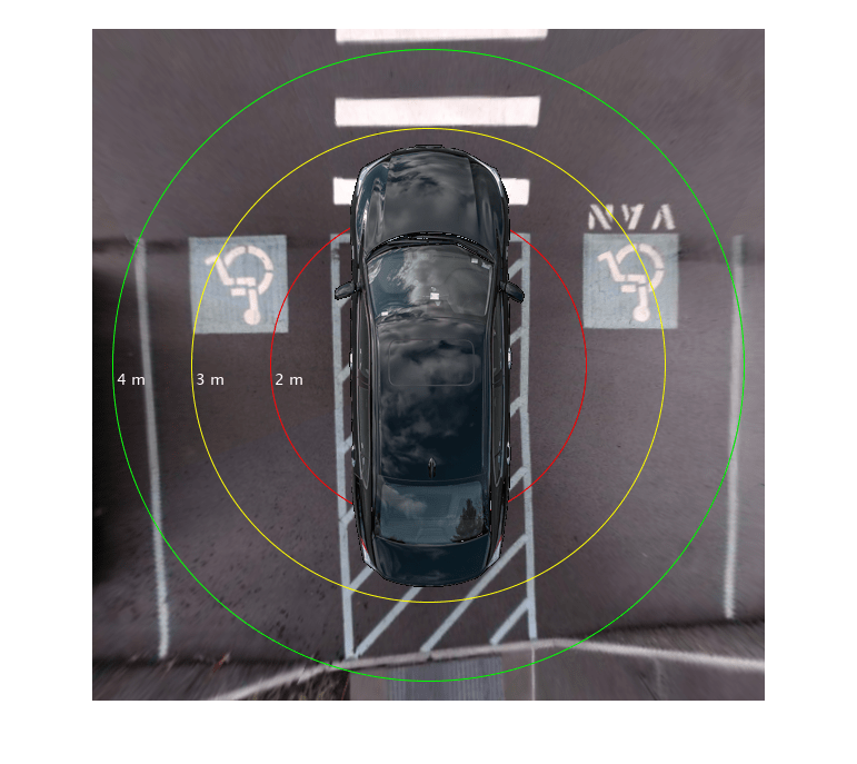
Code Generation and Verification
This algorithm can be deployed in hardware. To accomplish that, the next step is to package the proposed algorithm for generating 360° bird's-eye-view using images from eight surround cameras into a function, and generate code for it using MATLAB Coder™.
Restructure MATLAB Code for Code Generation
Following is a summary of the steps to generate 360° bird's-eye-view image, outlined in the previous sections:
Calibrate the multi-camera system and store the intrinsics and extrinsics in
monoCameraobjects.Obtain the bird's-eye-view transformations for each of the cameras and store them in
birdsEyeViewobjects.Transform the camera images into bird's-eye-view images and blend them to obtain the 360° surround view.
Register and stitch the corresponding camera images to generate the images of left and right-side views of the vehicle, and obtain the two respective transformations.
Obtain the final 360° bird's-eye-view image by registering and stitching the left and right side images of the vehicle.
Add circular guidelines at specific distances, overlay the simulated vehicle image on the bird's-eye-view image, and crop the final image to eliminate black borders.
However, the following additional considerations help restructure the above steps into the proposed algorithm for code generation:
Steps 1 and 2 need to be performed only once for a given stationary multi-camera setup. Hence, you can use the bird's-eye-view transformations obtained from MATLAB directly in the generated code.
Similarly, in step 4, you can use the two transformations for the left and right-side images obtained during the first-time setup in MATLAB, directly in the generated code. This eliminates the need to perform registration every time to generate the left and right-side images.
Applying the above considerations, this example provides helperGenerateBirdsEyeView, that serves as the entry-point function for code generation. The proposed algorithm in helperGenerateBirdsEyeView has the following steps:
Transform the current camera images to bird's-eye-view images using the
birdsEyeViewobjects.Obtain the left and right-side images of the vehicle using the respective transformations on the corresponding camera images.
Obtain the final 360° bird's-eye-view image by registering and stitching the left and right-side view images of the vehicle.
(Optional) Add circular guidelines at specific distances and overlay the simulated vehicle image on the bird's-eye-view image and crop the final image to eliminate black borders.
Generate Code and Verify Results
The entry-point function helperGenerateBirdsEyeView provides the final bird's-eye-view image overlayed with vehicle image as output. It has the following inputs:
sceneImages: Current camera images, specified as a cell array.intrinsicsStructs: cameraIntrinsicsobjects converted to structures, specified as a cell array of structures.bevStructs:BirdsEyeViewobjects converted to structures, specified as a cell array of structures.finalTforms: Transforms for left and right-side view images, specified as a cell array ofsimtform2dtransforms.egoVehicleImage: Simulated image of the ego vehicle to overlay on the final bird's-eye-view image, specified as M x N x 3 array.
To convert the cameraIntrinsics objects to structures, use helperToStructIntrinsics function. This gives us all the necessary inputs.
for i = 1:numCameras
    intrinsicsStructs{i} = helperToStructIntrinsics(intrinsics{i});
end
To convert the bird's-eye-view objects to structures, use helperToStructBev function. This gives us all the necessary inputs.
for i = 1:numCameras
    bevStructs{i} = helperToStructBev(birdsEye{i});
end
This example provides the MATLAB Coder project helper``GenerateBirdsEyeViewProject, that is already set up with the entry-point function, helperGenerateBirdsEyeView.
Click the project file. This opens the MATLAB Coder app in the toolstrip and MATLAB Coder panel on the right.
You can use the Prepare section of the toolstrip to define the input and output types and tune code generation settings.
The project is tuned for the build type to be MEX. This generates a MEX function, which is an executable for the generated code in MATLAB environment. This is useful to verify that the proposed algorithm provides the same functionality as the MATLAB code. In the toolstrip, navigate to the Generate Code and Build, and click Generate Code and Build from the drop-down. This will generate the MEX function.
After the code is generated, configure Verify Using MEX to execute the MEX function and verify the generated code output with the MATLAB algorithm output. In the drop-down, for Verification Mode, select Use Generated code. This calls the generated MEX function during testing. Click Run File and provide your own test function.
Alternatively, you can execute the MEX file directly by providing the same inputs as the entry-point function. Visualize the output image from the generated code and verify that it is the same as MATLAB code.
bevImage = helperGenerateBirdsEyeView_mex(sceneImages,intrinsicsStructs,bevStructs,finalTforms,egoVehicleImage);
imshow(bevImage)
For more information on authoring test functions for the generated code, see Unit Test Generated Code with MATLAB Coder (MATLAB Coder).
Conclusion
The procedure shown in this example can be extended to generate source code to deploy to the target hardware of a surround view monitoring system. For this, you must select the build type to be Source Code in the MATLAB Coder project and perform any necessary modifications to the MATLAB code. For more information, see Generate Deployable Standalone Code by Using the MATLAB Coder App (MATLAB Coder).
Note that this example requires accurate camera calibration to estimate the monocular camera positions with minimal errors and tuning the registration hyperparameters. This example can also be modified to use fisheye cameras.
Supporting Functions
helperVisualizeScene Function
The helperVisualizeScene function displays the images arranged by their camera positions relative to the vehicle on a 3-by-3 tiled chart layout and optionally shows the title text for each of the tiles.
helperBlendImages Function
The helperBlendImages function performs alpha blending to the given two input images, I1 and I2, with alpha values that are proportional to the center seam of each image. The output Iout is a linear combination of the input images:
helperRegisterImages Function
The helperRegisterImages function registers a cell array of images sequentially using the searching radius for matchFeaturesInRadius and returns the transformations, tforms.
helperStitchImages Function
The helperStitchImages function applies the transforms tforms to the input images and blends them to produce the outputImage. It additionally returns the outputView, which you can use to transform any point from the first image in the given image sequence to the output image.
helperVehicleToBirdsEyeView Function
The helperVehicleToBirdsEyeView function transforms the given world points in vehicle coordinate system to points in the 360° bird's-eye-view image.
helperGetImageBoundaryOnBEV Function
The helperGetImageBoundaryOnBEV function returns the position and size of a bounding box in the bird's-eye-view image that defines a square area that covers distFromVehicle meters around the vehicle.
helperGetVehicleBoundaryOnBEV Function
The helperGetVehicleBoundaryOnBEV function returns the corner points of a vehicle boundary given its position and size.
helperOverlayImage Function
The helperOverlayImage function overlays the topImage on the bottomImage and returns the result in outputImage.
helperGenerateBirdsEyeView Function
The helperGenerateBirdsEyeView function packages the bird's-eye-view generation logic into a MATLAB function for code generation.
helperToStructBev Function
The helperToStructBev function converts the specified birdsEyeView objects to structure format.
helperToObjectBev Function
The helperToObjectBev function creates birdsEyeView objects from the parameters specified in a structure format.
helperToStructIntrinsics Function
The helperToStructIntrinsics function converts the specified cameraIntrinsics objects to structure format.
helperToObjectIntrinsics Function
The helperToObjectIntrinsics function creates cameraIntrinsics objects from the parameters specified in a structure format.
See Also
Apps
Functions
undistortImage|estimateMonoCameraParameters|detectKAZEFeatures|matchFeatures|matchFeaturesInRadius|estgeotform3d