dsp.SineWave

R2026b

Generate discrete sine wave

Description

The dsp.SineWave System object™ generates a real or complex, multichannel sinusoidal signal with independent amplitude, frequency, and phase in each output channel.

For both real and complex sinusoids, the Amplitude, Frequency, and PhaseOffset properties can be scalars or length-N vectors, where N is the number of channels in the output. When you specify at least one of these properties as a length-N vector, scalar values specified for the other properties are applied to each of the N channels.

When you set the Method property to "Table lookup" and the TableOptimization property to "Speed", you can specify the frequency of the sine wave as any scalar or vector of scalars. The object generates a sine wave whose frequency is the closest achievable approximation using a table of length equal to the MaxTableLength property. (since R2026b)

The dsp.SineWave object and the sin function both generate a discrete sine wave signal. However, the object can process large streams of real-time data and handle system states automatically. The function performs one-time computations on readily available data and does not handle system states. For a comparison between the two, see System Objects vs MATLAB Functions.

To generate a discrete-time sinusoidal signal:

1. Create the dsp.SineWave object and set its properties.

2. Call the object with arguments, as if it were a function.

To learn more about how System objects work, see What Are System Objects?

Creation

Syntax

sine = dsp.SineWave

sine = dsp.SineWave(PropertyName=Value)

sine = dsp.SineWave(amp,freq,phase,PropertyName=Value)

Description

sine = dsp.SineWave creates a sine wave object that generates a real-valued sinusoid with an amplitude of 1, a frequency of 100 Hz, and a phase offset of 0. By default, the sine wave object generates only one sample.

sine = dsp.SineWave(PropertyName=Value) creates a sine wave object with each specified property set to the specified value. Enclose each property name in single quotes.

Example: sine = dsp.SineWave(Amplitude=2);

sine = dsp.SineWave(amp,freq,phase,PropertyName=Value) creates a sine wave object with the Amplitude property set to amp, Frequency property set to freq, PhaseOffset property set to phase, and any other specified properties set to the specified values.

Properties

Unless otherwise indicated, properties are nontunable, which means you cannot change their values after calling the object. Objects lock when you call them, and the release function unlocks them.

If a property is tunable, you can change its value at any time.

For more information on changing property values, see System Design in MATLAB Using System Objects.

Amplitude — Amplitude of sine wave

1 (default) | scalar | vector

Amplitude of the sine wave, specified as one of the following:

• scalar –– A scalar applies to all channels.

• vector –– A length-N vector contains the amplitudes of the sine waves in each of the N output channels. The vector length must be the same as that specified for the Frequency and PhaseOffset properties.

Tunable: Yes

Dependencies

This property is tunable only when you set Method to 'Trigonometric function' or "Differential".

Data Types: single | double | int8 | int16 | int32 | int64 | uint8 | uint16 | uint32 | uint64

Frequency — Frequency of sine wave

100 (default) | scalar | vector

Frequency of the sine wave in Hz, specified as one of the following:

• scalar –– A scalar applies to all channels.

• vector –– A length-N vector contains the frequencies of the sine waves in each of the N output channels. The vector length must be the same as that specified for the Amplitude and PhaseOffset properties.

Data Types: single | double | int8 | int16 | int32 | int64 | uint8 | uint16 | uint32 | uint64

PhaseOffset — Phase offset of sine wave

0 (default) | scalar | vector

Phase offset of the sine wave in radians, specified as one of the following:

• scalar –– A scalar applies to all channels.

• vector –– A length-N vector contains the phase offsets of the sine waves in each of the N output channels. The vector length must be the same as that specified for the Amplitude and Frequency properties.

Data Types: single | double | int8 | int16 | int32 | int64 | uint8 | uint16 | uint32 | uint64

ComplexOutput — Flag that indicates whether waveform is real or complex

false (default) | true

Flag that indicates whether the waveform is real or complex, specified as either:

• false –– The waveform output is real.

• true –– The waveform output is complex.

Method — Method used to generate sinusoids

"Trigonometric function" (default) | "Table lookup" | "Differential"

Method used to generate sinusoids, specified as one of the following:

• "Trigonometric function" –– The object computes the sinusoid by sampling the continuous-time function.

• "Table lookup" –– The object precomputes the unique samples of every output sinusoid at the start of the simulation, and recalls the samples from memory as needed.

• "Differential" –– The object uses an incremental algorithm. This algorithm computes the output samples based on the output values computed at the previous sample time and precomputed update terms.

TableOptimization — Table optimization for speed or memory

"Speed" (default) | "Memory"

Optimize table of sine values for speed or memory, specified as one of these:

• "Speed" –– The object precomputes a full table of sine values and recalls the samples from memory as needed. The object supports arbitrary frequencies and sample rates. If the frequency you specify is not exactly representable in the table, the object uses the closest achievable approximation using a table of length equal to the MaxTableLength property. Use the read-only ActualFrequency and FrequencyError properties to verify the generated frequency.

• "Memory" –– The table contains k/4 elements, where k is the number of input samples in one full period of the sine wave.

Dependencies

To enable this property, set the Method property to "Table lookup".

MaxTableLength — Maximum number of elements in the sine table

65535 (default) | positive integer

Since R2026b

Maximum number of elements in the sine table, specified as a positive integer less than or equal to 10⁷. The object uses a lookup table with at most this many elements to represent the sine wave. Increasing this value allows the object to represent more frequencies exactly, at the cost of additional memory.

For vector frequencies, this limit applies individually to each frequency.

Dependencies

To enable this property, set the Method property to "Table lookup" and the TableOptimization property to "Speed".

Data Types: single | double | int8 | int16 | int32 | int64 | uint8 | uint16 | uint32 | uint64

SamplesPerFrame — Number of samples per frame

1 (default) | positive integer

Number of consecutive samples from each sinusoid to buffer into the output frame, specified as a positive integer.

Data Types: single | double | int8 | int16 | int32 | int64 | uint8 | uint16 | uint32 | uint64

SampleRate — Sample rate of output signal

1000 (default) | positive scalar

Sample rate of output signal in Hz, specified as a positive scalar.

OutputDataType — Data type of the sine wave output

"double" (default) | "single" | "Custom"

Data type of the sine wave output, specified as "double", "single", or "Custom".

Read-Only Properties

TableLength — Actual number of elements in the sine table

Read-only: 10 (default) | positive integer | vector

Since R2026b

This property is read-only.

Table length for the generated sine wave, returned as a positive integer or a vector of length equal to the length of the Frequency vector. Each element in the vector corresponds to the table length used for the respective frequency in the Frequency property.

Dependencies

This property appears only when you set the Method property to "Table lookup" and the TableOptimization property to "Speed".

ActualFrequency — Actual frequency of generated sine wave

Read-only: 100 (default) | scalar | vector

Since R2026b

This property is read-only.

Actual frequency of the generated sine wave in Hz, returned as a scalar or a vector of length equal to the length of the Frequency vector. This is the closest representable frequency to the value you specify in the Frequency property, given the MaxTableLength constraint. The object wraps this value to the range [0, Fs).

Dependencies

This property appears only when you set the Method property to "Table lookup" and the TableOptimization property to "Speed".

FrequencyError — Difference between actual frequency and target frequency

Read-only: 0 (default) | scalar | vector

Since R2026b

This property is read-only.

Difference between the actual generated frequency and the specified target frequency in Hz, returned as a scalar or a vector of length equal to the length of the Frequency vector. A value of 0 indicates that the specified frequency is exactly representable in the table.

Dependencies

This property appears only when you set the Method property to "Table lookup" and the TableOptimization property to "Speed".

Fixed-Point Properties

CustomOutputDataType — Output word and fraction lengths

numerictype([],16) (default) | numerictype([],32,30)

Output word and fraction lengths, specified as an autosigned numeric type with a word length of 16.

Example: numerictype([],32,30)

Example: numerictype([],16,15)

Dependencies

This property applies only when you set the Method property to 'Table lookup' and the OutputDataType property to "Custom".

Usage

Syntax

sineOut = sine()

Description

sineOut = sine() creates the sine wave output, sineOut.

Output Arguments

sineOut — Sine wave output

vector | matrix

Sine wave output, returned as a vector or matrix. The SamplesPerFrame property determines the number of rows in the output matrix. If the Frequency or the PhaseOffset property is a vector, the length of the vector determines the number of columns (channels) in the output matrix. If the Frequency or the PhaseOffset property is a scalar, then the number of channels in the output matrix is 1.

The OutputDataType property sets the data type of the output.

Data Types: single | double | fi

Object Functions

To use an object function, specify the System object as the first input argument. For example, to release system resources of a System object named obj, use this syntax:

release(obj)

Common to All System Objects

step	Run System object algorithm
release	Release resources and allow changes to System object property values and input characteristics
reset	Reset internal states of System object

Examples

Generate a Sine Wave Signal

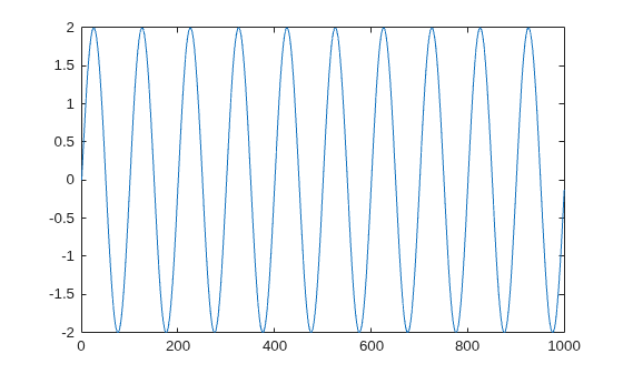
Generate a sine wave with an amplitude of 2, frequency of 10 Hz, and an initial phase of 0.

sine1 = dsp.SineWave(2,10);
sine1.SamplesPerFrame = 1000;
y = sine1();
plot(y)

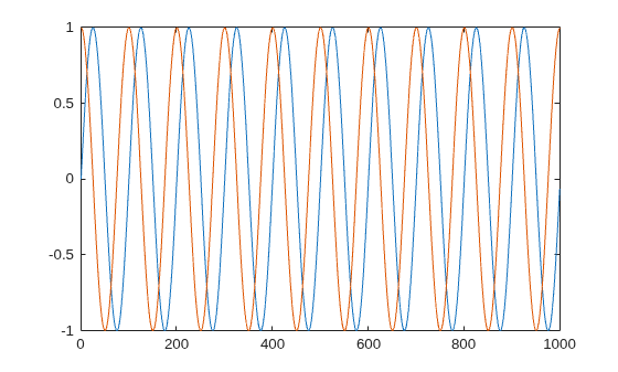
Generate two sine waves offset by a phase of pi/2 radians.

sine2 = dsp.SineWave;
sine2.Frequency = 10;
sine2.PhaseOffset = [0 pi/2];
sine2.SamplesPerFrame = 1000;
y = sine2();
plot(y)

Generate a Sine Wave Signal at an Arbitrary Frequency Using Table Lookup

Since R2026b

Generate a sine wave signal at an arbitrary frequency using the table look up method. For comparison, generate another sine wave signal at the same frequency using the trigonometric method. Use the time scope to compare the two signals.

Create Sine Wave Objects

Define the signal parameters. Use a frequency of $$\pi$$ Hz to demonstrate a frequency that is not exactly representable as a ratio of integers. Set the sample rate to 16 Hz, samples per frame to 256, and the number of frames to 200.

F = pi;
Fs = 16;
N = 256;
numFrames = 200;

Create a dsp.SineWave object. Choose the "Table lookup" method and set the TableOptimization to "Speed".

The speed-optimized table lookup method supports arbitrary frequencies by finding the closest representable frequency within a table of at most MaxTableLength elements, which is 65535 in this case.

sineLookup = dsp.SineWave(Frequency=F,SampleRate=Fs, ...
    SamplesPerFrame=N,Method="Table lookup",TableOptimization="Speed",...
    MaxTableLength=65535)

sineLookup = 
  dsp.SineWave with properties:

            Amplitude: 1
            Frequency: 3.1416
          PhaseOffset: 0
        ComplexOutput: false
               Method: 'Table lookup'
    TableOptimization: 'Speed'
       MaxTableLength: 65535
      SamplesPerFrame: 256
           SampleRate: 16
       OutputDataType: 'double'

  Show all properties

View the actual frequency of the generated sine wave, the error between the target frequency ($$\pi$$ Hz) and the actual frequency, and the table length the object uses to generate the sine wave.

fprintf("Target frequency: %.6f Hz\n",F)

Target frequency: 3.141593 Hz

fprintf("Actual frequency:    %.6f Hz\n",sineLookup.ActualFrequency)

Actual frequency:    3.141593 Hz

fprintf("Frequency error:     %.2e Hz\n",sineLookup.FrequencyError)

Frequency error:     -3.34e-09 Hz

fprintf("Table length:        %d samples\n",sineLookup.TableLength)

Table length:        32763 samples

Create a second dsp.SineWave object and set the Method to "Trigonometric function".

sineTrig = dsp.SineWave(Frequency=F,SampleRate=Fs, ...
    SamplesPerFrame=N,Method="Trigonometric function")

sineTrig = 
  dsp.SineWave with properties:

          Amplitude: 1
          Frequency: 3.1416
        PhaseOffset: 0
      ComplexOutput: false
             Method: 'Trigonometric function'
    SamplesPerFrame: 256
         SampleRate: 16
     OutputDataType: 'double'

Create a timescope object to compare the two sinusoidal signals over time.

scope = timescope(SampleRate=Fs, ...
    TimeSpanSource="property", ...
    TimeSpan=numFrames*N/Fs, ...
    TimeSpanOverrunAction="Scroll", ...
    ShowGrid=true, ...
    ChannelNames=["Trigonometric","Table Lookup"], ...
    Title="Deviation from Baseline");

Generate Sine Waves and Compare Deviation from Baseline

Generate the two sine wave signals. To compare these two signals, first compute the deviation of these signals from a high-precision baseline. To compute the baseline, use the sinpi function. Visualize the deviation of these signals from the baseline using the time scope.

[num,den] = rat(sineLookup.ActualFrequency/Fs,0);
for k = 1:numFrames
    yLookup = sineLookup();
    yTrig = sineTrig();
    idx = (k-1)*N + (0:N-1)';
    baseline = sinpi(2*mod(num*idx,den)/den);
    scope([yTrig-baseline, yLookup-baseline])
end

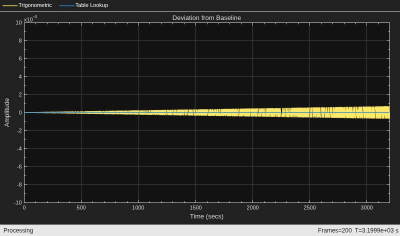
Zoom in on the deviation plot. The table lookup method generates a sine wave that closely mimics the baseline and does not aggregate any noticeable cumulative error over time. The trigonometric method generates a sine wave that accumulates numeric error which grows over time.

scope.YLimits = [-10e-4 10e-4]

scope = 
  timescope handle with properties:

               SampleRate: 16
           TimeSpanSource: 'property'
                 TimeSpan: 3200
    TimeSpanOverrunAction: 'scroll'
              YLimitsMode: 'manual'

  Show all properties

Increase Maximum Table Length for Better Accuracy

To reduce the error between the target frequency and the generated frequency, increase the MaxTableLength property value to allow a longer table. A longer table can represent the frequencies more precisely.

With a MaxTableLength of 65535 elements, the frequency error is $-3.34e^{-9}$ Hz. Increase the MaxTableLength to $1e^6$.

release(sineLookup)
sineLookupLargeTable = dsp.SineWave(Frequency=F,SampleRate=Fs, ...
    SamplesPerFrame=N,Method="Table lookup",MaxTableLength=1e6)

sineLookupLargeTable = 
  dsp.SineWave with properties:

            Amplitude: 1
            Frequency: 3.1416
          PhaseOffset: 0
        ComplexOutput: false
               Method: 'Table lookup'
    TableOptimization: 'Speed'
       MaxTableLength: 1000000
      SamplesPerFrame: 256
           SampleRate: 16
       OutputDataType: 'double'

  Show all properties

With an increased table length, the frequency of the generated sine wave now has more precision.

sineLookupLargeTable.ActualFrequency

ans = 
3.1416

The frequency error reduces to $1.61e^{-12}$ Hz. The object uses a table of length 729826 samples. Increasing the maximum table length reduces the frequency error at the cost of additional memory.

sineLookupLargeTable.FrequencyError

ans = 
1.6107e-12

sineLookupLargeTable.TableLength

ans = uint32

729826

Filter Frames of a Noisy Sine Wave Signal in MATLAB

This example shows how to lowpass filter a noisy signal in MATLAB® and visualize the original and filtered signals using a spectrum analyzer. For a Simulink® version of this example, see Filter Frames of a Noisy Sine Wave Signal in Simulink.

Specify Signal Source

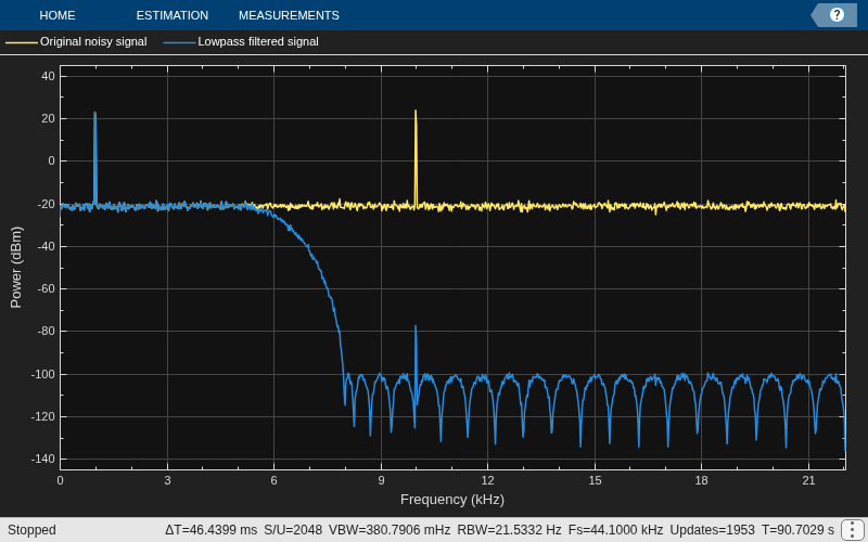
The input signal is the sum of two sine waves with frequencies of 1 kHz and 10 kHz. The sampling frequency is 44.1 kHz.

Sine1 = dsp.SineWave(Frequency=1e3,SampleRate=44.1e3);
Sine2 = dsp.SineWave(Frequency=10e3,SampleRate=44.1e3);

Create Lowpass Filter

The lowpass FIR filter, dsp.LowpassFilter, designs a minimum-order FIR lowpass filter using the generalized Remez FIR filter design algorithm. Set the passband frequency to 5000 Hz and the stopband frequency to 8000 Hz. The passband ripple is 0.1 dB and the stopband attenuation is 80 dB.

FIRLowPass = dsp.LowpassFilter(PassbandFrequency=5000,...
    StopbandFrequency=8000);

Create Spectrum Analyzer

Set up the spectrum analyzer to compare the power spectra of the original and filtered signals. The spectrum units are dBm.

SpecAna = spectrumAnalyzer(PlotAsTwoSidedSpectrum=false,...
    SampleRate=Sine1.SampleRate,...
    ShowLegend=true, ...
    YLimits=[-145,45]);

SpecAna.ChannelNames = {"Original noisy signal",...
    "Lowpass filtered signal"};

Specify Samples per Frame

This example uses frame-based processing, where data is processed one frame at a time. Each frame of data contains sequential samples from an independent channel. Frame-based processing is advantageous for many signal processing applications because you can process multiple samples at once. By buffering your data into frames and processing multisample frames of data, you can improve the computational time of your signal processing algorithms. Set the number of samples per frame to 4000.

Sine1.SamplesPerFrame = 4000;
Sine2.SamplesPerFrame = 4000;

Filter the Noisy Sine Wave Signal

Add zero-mean white Gaussian noise with a standard deviation of 0.1 to the sum of sine waves. Filter the result using the FIR filter. While running the simulation, the spectrum analyzer shows that frequencies above 8000 Hz in the source signal are attenuated. The resulting signal maintains the peak at 1 kHz because it falls in the passband of the lowpass filter.

for i = 1 : 1000
    x = Sine1()+Sine2()+0.1.*randn(Sine1.SamplesPerFrame,1);
    y = FIRLowPass(x);    
    SpecAna(x,y);                              
end
release(SpecAna)

Bandpass Filtering of Sinusoids

Bandpass filter a discrete-time sine wave signal which consists of three sinusoids at frequencies, 1 kHz, 10 kHz, and 15 kHz.

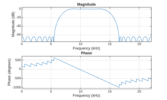
Design an FIR Equiripple bandpass filter by first creating a bandpass filter design specifications object, and then designing a filter using these specifications.

Design Bandpass Filter

Create a bandpass filter design specifications object using fdesign.bandpass.

bandpassSpecs = fdesign.bandpass('Fst1,Fp1,Fp2,Fst2,Ast1,Ap,Ast2', ...
    1/4,3/8,5/8,6/8,60,1,60);

List the available design methods for this object.

designmethods(bandpassSpecs)

Design Methods for class fdesign.bandpass (Fst1,Fp1,Fp2,Fst2,Ast1,Ap,Ast2):


butter
cheby1
cheby2
ellip
equiripple
kaiserwin

To design an Equiripple filter, pick 'equiripple'.

bpFilter = design(bandpassSpecs,'equiripple',Systemobject=true)

bpFilter = 
  dsp.FIRFilter with properties:

            Structure: 'Direct form'
      NumeratorSource: 'Property'
            Numerator: [-0.0043 -3.0812e-15 0.0136 3.7820e-15 -0.0180 -4.2321e-15 7.1634e-04 4.0993e-15 0.0373 -4.1057e-15 -0.0579 3.7505e-15 0.0078 -3.4246e-15 0.1244 2.4753e-15 -0.2737 -8.6287e-16 0.3396 -8.6287e-16 -0.2737 2.4753e-15 … ] (1×37 double)
    InitialConditions: 0

  Show all properties

Visualize the frequency response of the designed filter.

freqz(bpFilter,[],44100)

Create Sinusoidal Signal

Create a signal that is a sum of three sinusoids with frequencies at 1 kHz, 10 kHz, and 15 kHz. Initialize spectrum analyzer to view the original signal and the filtered signal.

Sine1 = dsp.SineWave(Frequency=1e3,SampleRate=44.1e3,SamplesPerFrame=4000);
Sine2 = dsp.SineWave(Frequency=10e3,SampleRate=44.1e3,SamplesPerFrame=4000);
Sine3 = dsp.SineWave(Frequency=15e3,SampleRate=44.1e3,SamplesPerFrame=4000);

SpecAna = spectrumAnalyzer(PlotAsTwoSidedSpectrum=false, ...
    SampleRate=Sine1.SampleRate, ...
    ShowLegend=true, ...
    YLimits=[-240,45]);

SpecAna.ChannelNames = {'Original noisy signal','Bandpass filtered signal'};

Filter Sinusoidal Signal

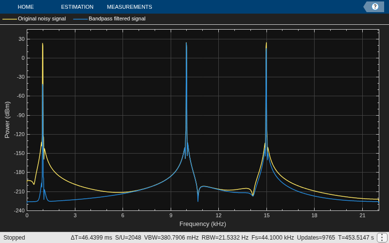
Filter the sinusoidal signal using the bandpass filter that has been designed. View the original signal and the filtered signal in the spectrum analyzer. The tone at 1 kHz is filtered out and attenuated. The tone at 10 kHz is unaffected, and the tone at 15 kHz is mildly attenuated because it appears in the transition band of the filter.

for i = 1:5000
    x = Sine1()+Sine2()+Sine3();
    y = bpFilter(x);
    SpecAna(x,y);
end
release(SpecAna)

More About

Sinusoid

A real-valued, discrete-time sinusoid is defined as:

$$y(n)=A\sin (2\pi fn+\varphi )$$

where A is the amplitude, f is the frequency in Hz, and φ is the initial phase, or phase offset, in radians.

A complex sinusoid is defined as:

$$y(n)=A{e}^{j(2\pi fn+\varphi )}$$

Algorithms

Trigonometric Function

The trigonometric function method computes the sinusoid in the ith channel, y_i, by sampling the continuous function

$$\begin{array}{ll}{y}_i=A_i\sin \left(2\pi f_{i}t+{\varphi }_i\right)\hfill & \text{(real)}\hfill \\ \begin{array}{l}\\ \text{or}\\ \end{array}\hfill & \hfill \\ y_i=A_i{e}^{j\left(2\pi f_{i}t+{\varphi }_i\right)}\hfill & \text{(complex)}\hfill \end{array}$$

with a period of T_s, where you specify T_s in the sample time.

At each sample time, the algorithm evaluates the sine function at the appropriate time value in the first cycle of the sinusoid. By constraining trigonometric evaluations to the first cycle of each sinusoid, the algorithm avoids the imprecision of computing the sine of very large numbers. This constraint also eliminates the possibility of discontinuity during extended operations, when an absolute time variable might overflow. This method therefore avoids the memory demands of the table lookup method at the expense of many more floating-point operations.

Table Lookup

The table lookup method precomputes the unique samples of every output sinusoid at the start of the simulation, and recalls the samples from memory as needed.

When the algorithm optimizes the table for Speed, the object supports arbitrary frequencies and sample rates. The object finds the closest representable frequency in a table of at most MaxTableLength elements. The algorithm uses rational approximation to determine the optimal table length and stride, then refines the result by searching for a better representation within the maximum table length constraint. The generated sinusoid is periodic and repeatable after a certain number of periods, with no cumulative numeric error. (since R2026b)

When the algorithm optimizes the table for Memory, the table constructed for each channel contains k_i/4 elements, where k_i is the number of input samples in one full period of the sine wave. The Memory optimization requires that the period of every sinusoid in the output be evenly divisible by the sample period.

For long output sequences, the table lookup method requires far fewer floating-point operations than any of the other methods. However, the method can demand considerably more memory, especially for high sample rates (long tables). Use this method for models that emulate or generate code for DSP hardware that you want to optimize for execution speed.

Note

The lookup table for this object is constructed from double-precision floating-point values. When you use the Table Lookup computation mode, the maximum amount of precision you can achieve in your output is 53 bits. Setting the word length of the output data type to values greater than 53 bits does not improve the precision of your output.

Differential

The differential method uses an incremental algorithm. This algorithm computes the output samples based on the output values computed at the previous sample time (and precomputed update terms) by making use of the following identities.

$$\begin{array}{l}\sin \left(t+T_s\right)=\sin \left(t\right)\cos \left(T_s\right)+\cos \left(t\right)\sin \left(T_s\right)\\ \cos \left(t+T_s\right)=\cos \left(t\right)\cos \left(T_s\right)-\sin \left(t\right)\sin \left(T_s\right)\end{array}$$

The update equations for the sinusoid in the ith channel, y_i, can therefore be written in matrix form as

$$\left[\begin{array}{c}\sin \left\{2\pi f_i\left(t+T_s\right)+{\varphi }_i\right\}\\ \cos \left\{2\pi f_i\left(t+T_s\right)+{\varphi }_i\right\}\end{array}\right]=\left[\begin{array}{cc}\cos \left(2\pi f_i{T}_s\right)& \sin \left(2\pi f_i{T}_s\right)\\ -\sin \left(2\pi f_i{T}_s\right)& \cos \left(2\pi f_i{T}_s\right)\end{array}\right]\left[\begin{array}{c}\sin \left(2\pi f_{i}t+{\varphi }_i\right)\\ \cos \left(2\pi f_{i}t+{\varphi }_i\right)\end{array}\right]$$

where you specify T_s in the sample time. Because T_s is constant, the right-side matrix is a constant and can be computed once at the start of the simulation. The value of A_isin[2πf_i(t+T_s)+ϕ_i] is then computed from the values of sin(2πf_it+ϕ_i) and cos(2πf_it+ϕ_i) by a simple matrix multiplication at each time step.

This mode offers reduced computational load, but can drift over time due to cumulative quantization error. Because the method is not contingent on an absolute time value, there is no danger of discontinuity during extended operations, when an absolute time variable might overflow.

Extended Capabilities

C/C++ Code Generation

Generate C and C++ code using MATLAB® Coder™.

Usage notes and limitations:

• This object has no tunable properties for code generation.

• See System Objects in MATLAB Code Generation (MATLAB Coder).

Version History

Introduced in R2012a

R2026b: Support for arbitrary frequencies in table lookup mode

When you set the Method property to "Table lookup" and the TableOptimization property to "Speed", you can specify any scalar or vector of scalars for the Frequency property and any positive scalar for the SampleRate property.

If the frequency you specify is not exactly representable in the table, the object uses the closest achievable approximation based on a lookup table of length MaxTableLength. Use the read-only ActualFrequency and FrequencyError properties to verify the generated frequency.

Here are the new properties that support the table lookup method.

• MaxTableLength — Maximum number of elements in the precomputed sine table.

• TableLength — Read-only field that displays the actual table length.

• ActualFrequency — Read-only field that displays the actual frequency of the generated sine wave.

• FrequencyError — Read-only property that reports the difference between the actual frequency and the specified frequency.

Existing code that uses table lookup mode continues to produce numerically identical results when the default maximum table length remains unchanged.