Time Delay and Scaling in Multirate DSP Filters
This example demonstrates the effect of time delay and scaling in multirate filters, and how to calculate them.
Time Delay and Scaling Model in Multirate Filters
A multirate filter is a cascade combining upsampling, downsampling, and convolution filters (FIR or IIR). Such filter structures are often used to implement resampling systems, wherein the output is a resampled version of the input at a different rate. Informally, for an input , the output of a resampling system is . This is stated with a slight abuse of notations, since is undefined when is noninteger. More formally, the input is interpolated to a continuous domain function from which the output is sampled:
.
The input can sometimes be approximated by sampling at the input rate . Approximation is used instead of equality due to the filtering operation (e.g. lowpass/highpass) which is an integral part of the interpolation model. The interpolation model does not necessarily preserve the values of every input .
The constants , and in the equations above are the input sample rate, output sample rate, and the resampling output delay respectively. For many multirate filtering applications, it is useful to find and for a given input sample rate .
Using the outputDelay Function
You can use the outputDelay function to calculate the resampling output delay and output sample rate for a given filter object operating at a given input sample rate. This function is available for any DSP System object that supports filter analysis methods. For a list of supported objects, refer to the outputDelay function. The returned delay value is specified in the natural units of the interpolated signal (usually seconds), corresponding to the same units as the input sample rate.
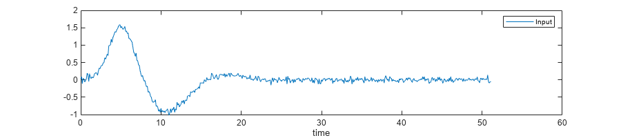
Consider a signal that is sampled from a continuous signal at a rate of Ts=0.1s (that is, Fs=10 Hz). Add zero-mean white Gaussian noise with a standard deviation of 0.05.
f = analyticSignal(); % x is a function of a real variable
Ts = 1/10;

n = (0:511)'; % Sample index vector
u = f(n*Ts)+0.05*randn(size(n));

figure(Position=[0 0 900 200])
plot(n*Ts,u)
xlabel("Time")
legend("Input")
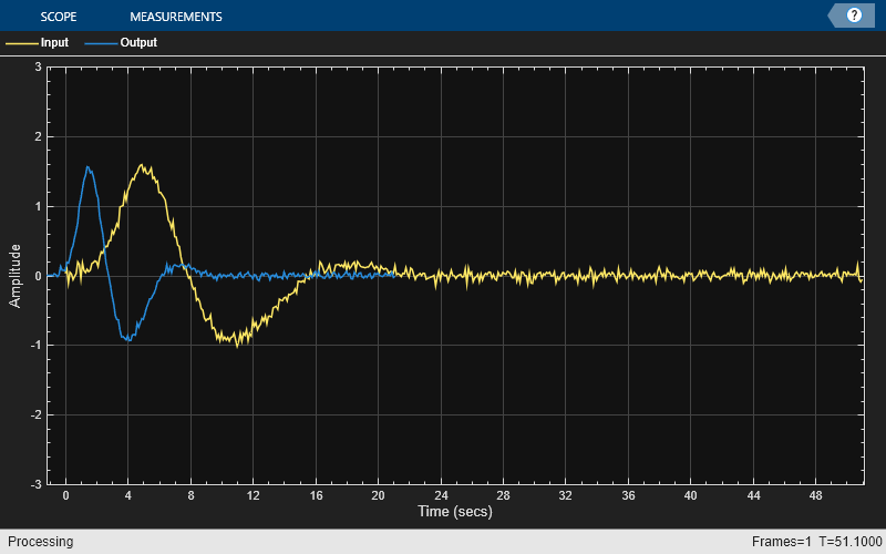
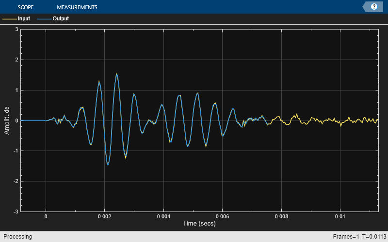
To eliminate the high frequency noise, design a lowpass filter and apply it to the signal. This lowpass has a cutoff at 15% of the Nyquist frequency with a transition width of 10%. Plot the input against the filtered output on the same graph. Note the delay between the input and the filtered signal.
Fs = 1/Ts;
Fnyq = Fs/2;
F0 = 0.15;    % Cutoff frequency normalized to the Nyquist frequency
TW = 0.1;
g1 = dsp.LowpassFilter(SampleRate=Fs, ...
                    PassbandFrequency=(F0-TW/2)*Fnyq, ...
                    StopbandFrequency=(F0+TW/2)*Fnyq);
y = g1(u);
ts = timescope(SampleRate=Fs, ...
               ChannelNames=["Input" "Lowpass Output"],...
               YLimits=[-3 3]);
ts(u,y)
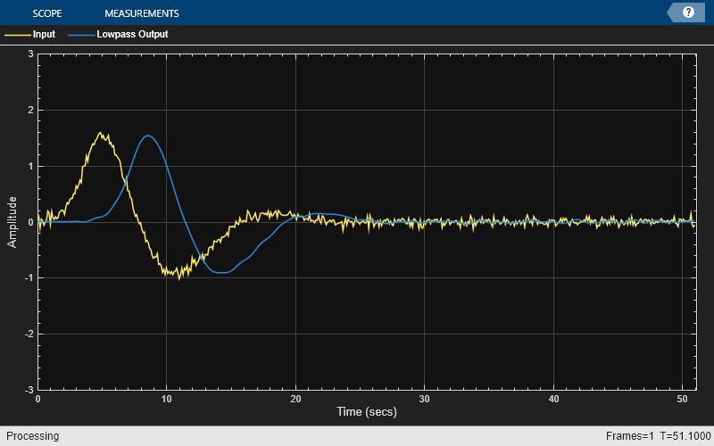
The observed delay is inherent to any convolution filter, such as the one implemented in dsp.LowpassFilter. Call the outputDelay function to find that output delay.
D = outputDelay(g1)
D =
3.6000
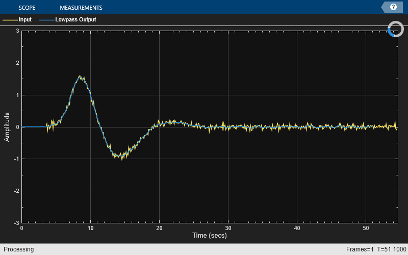
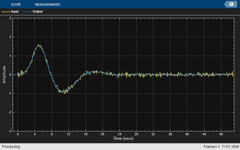
To align the input with the output, shift the output back in time by D units, of shift the input forward in time by the same amount. You can perform such a shift using the TimeDisplayOffset property of the timescope object. When you specify a vector in TimeDisplayOffset instead of a scalar, each input channel of the timescope object has its own delay, corresponding to the entries of the vector in TimeDisplayOffset. Set the first channel (input) delay to D, and keep the second channel (output) with no delay. The two channels are now synchronized.
release(ts)
ts.TimeDisplayOffset = [D 0];
ts(u,y)
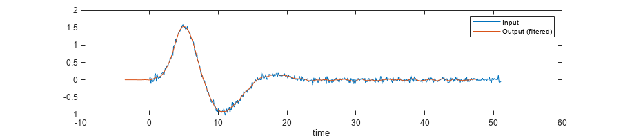
The same delay can be used with standard MATLAB® plots.
plot(n*Ts,u)
hold on
plot(n*Ts-D,y)
hold off
xlabel("Time")
legend("Input","Output (filtered)")
The Relation Between Resampling Output Delay and the Group Delay
The outputDelay function uses the group delay of the convolution stages to calculate the overall resampling output delay. Although the two terms are closely related, there are several distinctions between the two:
Scalar vs a function: Group delay is a function of frequency, defined as where is the phase response of a convolution system. Output delay is defined as a scalar, and it stems from the resampling model .
Scope of definition: Output delay applies to multirate filters, whereas group delay is well defined only for convolution systems (single-rate LTI systems).
Units: Group delay is measured in sample units. Output delay is defined in time units of the interpolated signal
When the convolution stages of a multirate filter have a linear phase, their group delays do not depend on the input frequency. Symmetric filter designs, which are very common in DSP applications, have a linear phase. In the simple case of a single-stage symmetric convolution filter, the output delay is merely the (constant) group delay scaled to the sample time, i.e. . For a single-stage filter with a nonlinear phase, the output delay depends on the input frequency, namely . For a multistage filter, the output delay is the sum of output delays of its stages. The multi-stage and nonlinear phase cases will be discussed later in this example.
In the simple case of a symmetric single-stage filter, the group delay can be thought of as the center of mass of its impulse response, which is its point of symmetry. The filter g1 in the example above is a 73-taps FIR, symmetric about its 36th index.
h = impz(g1);
stem(0:length(h)-1,h)
hold on
xline(36,Color="red")
hold off
xlabel("n (samples)")
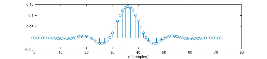
The filter introduces a group delay of 36 samples, which is equivalent to an output delay of 3.6 time units accounting for the sample rate Fs=10 Hz. Calculate the output delay using center-of-mass weighted sum formula and verify that it is indeed 3.6, the exact same value returned from outputDelay.
D_cm = Ts*sum((0:length(h)-1)'.*h)/sum(h)
D_cm =
3.6000
Working with Sample Rates
You can specify or override the input sample rate by using the named argument InputSampleRate. For example, calculate the output delay assuming that the input sample rate is 2 kHz instead of 10 Hz. Note that the returned delay value changes accordingly to reflect the new time units.
D2k = outputDelay(g1,InputSampleRate=2e3) % Override the sample rate to 2 kHzD2k = 0.0180
If InputSampleRate argument is unspecified, the input sample rate is obtained from the object on which outputDelay is called. If the object has an intrinsic sample rate property, InputSampleRate equals that property. For example, dsp.LowpassFilter and dsp.IIRHalfbandDecimator have the property SampleRate, and dsp.FarrowRateConverter has the property InputSampleRate. Objects without such a property which contain filter design data (such as objects that were designed using designfilt) can still provide an input sample rate. For objects that do not have a sample rate property, such as dsp.FIRFilter and dsp.FIRDecimator, the default value for InputSampleRate is 1 (one sample per second).
Obtaining the Output Sample Rate of a Multirate Filter
Multirate filters such as dsp.FIRRateConverter often involve rate change, so the input sample rate and output sample rate are not equal. In the following example, the output appears shrank on the time domain.
g2 = dsp.FIRRateConverter(7,16);
y = g2(u);

D  = outputDelay(g2,InputSampleRate=Fs);
ts = timescope(SampleRate=Fs, ...
                TimeDisplayOffset=[0 -D],...
                ChannelNames=["Input" "Output"],...
                YLimits=[-3 3]);
ts(u,y)
The outputDelay function returns the output sample rate as the second output argument, which is particularly convenient when using dsp.FilterCascade objects. Call outputDelay with two output arguments to obtain .
[D,FsOut] = outputDelay(g2,InputSampleRate=Fs)
D =
1.2000
FsOut =
4.3750
You can specify different sample rates for each channel of a timescope object, by setting a vector to its SampleRate property instead of a scalar. Make sure to use the same channel order as you step through the timescope object. Set the first entry of SampleRate to Fs (the input sample rate), and the second to FsOut (the output sample rate). The input and output now have the same scale on the plot.
ts = timescope(SampleRate=[Fs FsOut], ...
                 TimeDisplayOffset=[0 -D],...
                 ChannelNames=["Input" "Output"],...
                 YLimits=[-3 3]);
ts(u,y)
Bandlimited Mode: Using outputDelay with Nonlinear Phase Filters
So far, we used symmetric filter designs, which have a linear phase, and a constant group delay. Asymmetric filters, on the other hand, have a varying group delay and can exhibit signal distortion in the time domain, which breaks the resampling model described above. Using outputDelay in such cases is possible, but requires some caution. This is discussed in the next section.
Distortion in Nonlinear Phase Filters
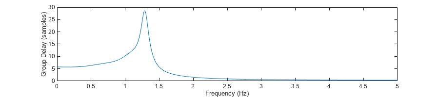
Causal and stable rational IIR filters are common in DSP, and they often have a nonlinear phase. For example, consider the following lowpass IIR design, which clearly has a varying group delay.
F0 = 0.35;
TW = 0.2;
g3 = dsp.LowpassFilter(SampleRate=Fs, ...
                    PassbandFrequency=(F0-TW/2)*Fnyq, ...
                    StopbandFrequency=(F0+TW/2)*Fnyq, ...
                    FilterType="IIR");
grpdelay(g3,2048,Fs)
The outputDelay function alerts the user if the system has a nonlinear phase convolution stage.
>> D  = outputDelay(g3); % Throws a warning.
% The System object has a nonlinear phase, but a carrier frequency Fc has not been specified.
% To suppress this warning, specify Fc argument explicitly, or call the outputDelay method with
% band measurement output. If you don't specify any value, the default carrier frequency is Fc=0.
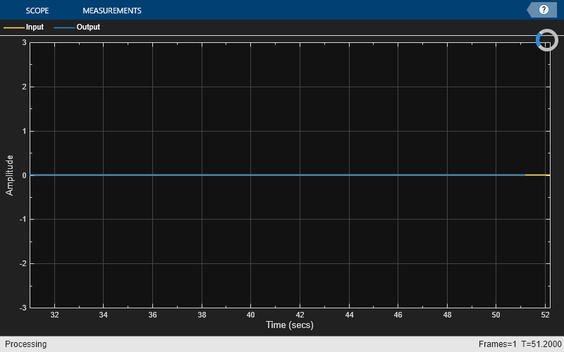
To demonstrate the effect of a nonlinear phase distortion, input a short time pulse to the IIR filter g3. Note that the input and the output are not related by a time delay and scaling, i.e. they no longer satisfy the resampling model and .
v = f(10*Ts*n);
y = g3(v);

release(ts)
ts.TimeDisplayOffset = [D 0];
ts(v(1:128),y(1:64))
Using outputDelay on a filter with nonlinear phase stages only makes sense if the group delay of the stages is relatively constant on the input signal band. That could happen if:
The filter stages have a flat group delay response over a known band, or
If the input is narrowband, so that the group delay response can be approximated as a constant on the input band.
In any case, since the group delay is not constant, you need to specify the frequency from which the group delay is sampled. The outputDelay function accepts this frequency (specified in input sample rate units) through the parameter CarrierFrequency.
Nonlinear Phase Filters with a Partially Flat Group Delay Response (Quasi-Linear Phase)
Some filter designs have a nonlinear phase, yet still have a relatively flat group delay on subbands. For example, any FIR designed using the designFracDelayFIR function has a relatively flat group delay. Another example is the quasi-linear-phase designs generated by the designHalfbandIIR function. The quasi-linear design algorithm compensates for the nonlinear phase of the IIR on the passband and considerably reduces the distortion.
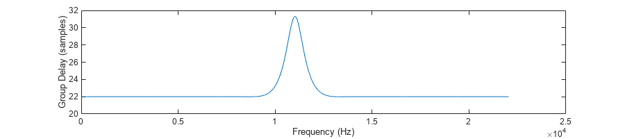
Design an IIR halfband decimator, and plot its group delay. The group delay is obviously not constant, yet relatively flat outside the transition band.
Fs=44100;
g4 = designHalfbandIIR(InputSampleRate=Fs,...
                       TransitionWidth=Fs/10,StopbandAttenuation=80,...
                       DesignMethod="quasilinphase",SystemObject=true);

grpdelay(g4,8192,Fs)
ylim([17 30])
To obtain the output delay for a bandlimited signal on the flat region, set CarrierFrequency to be any frequency within that flat region. Note that a slight deviation of the delay values of different frequencies within the flat region is normal and is expected.
D1 = outputDelay(g4,CarrierFrequency=0)
D1 =
4.5354e-04
Fc = 5000;
D2 = outputDelay(g4,CarrierFrequency=Fc) % 5 kHz is still in the flat region
D2 = 4.5349e-04
Input Band Measurement
For a filter with nonlinear phase stages, changing CarrierFrequency affects the output delay D. The outputDelay function can calculate the interval of input frequencies B = [f1, f2] around CarrierFrequency that have a delay value close to D up to a tolerance, or for every . The edges of the band, f1 and f2, are returned in the third output argument of the outputDelay function. The tolerance is specified in sample time units using the Tolerance named parameter. For example, obtain the input frequency band for which the delay deviates by up to Tolerance = 1 second from the nominal value D at the frequency CarrierFrequency.
[D, ~, B] = outputDelay(g4,CarrierFrequency=Fc,Tolerance=1) % Discard FsOut output argumentD = 4.5349e-04
B = 1×2
103 ×

   -9.8568    9.8568
Note that the measured band is two-sided and might contain negative frequencies.
[G, W] = grpdelay(g4,8192,Fs);
I = W>=B(1) & W<=B(2); % Find band indices

plot(W/1e3,G)
xlabel("Frequency (kHz)")
ylabel("Group Delay (samples)")
hold on
scatter(Fc/1e3,D*Fs,"filled")
plot(W(I)/1e3,G(I),LineWidth=3)
xline(Fc/1e3)
hold off
legend("Group delay","Fc","Applicable band for Tolerance=1")
grid on
ylim([17 30])
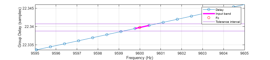
Band Measurement Resolution
If the tolerance value of the band measurement is very low, the resulting band may be a singleton (contains a single frequency, the specified frequency Fc), which is a degenerate case. This is because the group delay search resolution is too coarse for the specified tolerance. For example, repeat the band measurement of the system g4 with a tight tolerance of Tolerance = 1e-3. The returned B equals to [Fc, Fc], indicating that is has a single frequency.
Fc  = 9600;
Tol = 1e-3;
[D, ~, B] = outputDelay(g4,CarrierFrequency=Fc,Tolerance=Tol);
D
D =
4.6410e-04
plot(W/1e3,G,"-o")
xlabel("Frequency (kHz)")
ylabel("Group Delay (samples)")
hold on
scatter(Fc/1e3,D*Fs,"filled")
yline(D*Fs+[-Tol Tol],Color=[0.5 0 0.8])
xline(Fc/1e3)
legend("Group delay","Fc","Tolerance interval")
grid on
hold off
xlim([Fc-5 Fc+5]/1e3)
An obvious solution is to relax the tolerance. However, if you want to keep the low tolerance, you can instead increase the group delay resolution by using the FFTLength parameter. The default length is . Increase FFTLength to and notice that the returned B has two distinct edges, and not a single frequency.
[D, ~, B] = outputDelay(g4,CarrierFrequency=Fc,Tolerance=Tol,FFTLength=2^16)
D =
4.6410e-04
B = 1×2
103 ×

    9.5998    9.6004
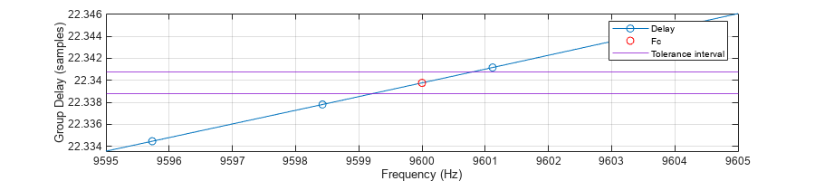
To plot the band, calculate the group delay with increased resolution as well.
[G, W] = grpdelay(g4,2^16,"whole",Fs);
I = W>=B(1) & W<=B(2); % Find band indices
plot(W/1e3,G,"-o")
xlabel("Frequency (kHz)")
ylabel("Group Delay (samples)")
hold on
scatter(Fc/1e3,D*Fs,"filled")
plot(W(I)/1e3,G(I),LineWidth=3)
yline(D*Fs+[-Tol Tol],Color=[0.5 0 0.8])
xline(Fc/1e3)
legend("Group delay","Fc","Input band","Tolerance interval");
grid on
hold off
xlim([Fc-5 Fc+5]/1e3)
Narrowband Signals
The outputDelay function can be used even if the group delay is not flat, given that the input signal is a narrowband signal. The band measurement returned from outputDelay can be used to determine the maximal bandwidth for the signal subject to a delay tolerance.
When the system under consideration has a nonlinear phase and the signal is narrowband signal centered around some carrier frequency , the resampling model is slightly different than in the linear phase case. The input is approximated by
,
and the output is
.
The base band signal is delayed by the output delay , which is calculated using the group delay obtained from . The carrier signal, however, experiences a different delay, called phase delay, and denoted . For single-rate systems, the phase delay is merely the negative of the system's phase response measured at and divided by .
.
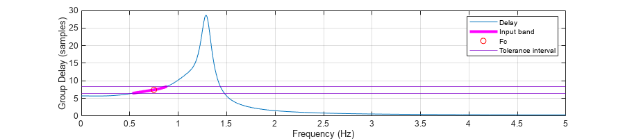
Consider the IIR design g3, and obtain the output delay for a narrowband signal with the center frequency Fc=0.75 Hz. Indeed, the returned band B=[0.526 Hz, 0.885 Hz] contains the carrier frequency, and has a bandwidth of 0.3589 Hz.
Fs = g3.SampleRate;
Ts = 1/Fs;
Fnyq = Fs/2;
Fc  = 0.15*Fnyq;
Tol = 1; % Deviation up to 1 time unit
[D, ~, B] = outputDelay(g3,InputSampleRate=Fs,CarrierFrequency=Fc,Tolerance=Tol)
D = 0.7457
B = 1×2

    0.5261    0.8850
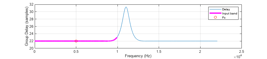
Plot the response and the band, and verify that the frequency Fc is indeed contained in the band.
[G, W] = grpdelay(g3,2048,Fs);
Fc = 0.15*Fnyq; % Carrier frequency
I = W>=B(1) & W<=B(2); % Find band indices

plot(W/1e3,G)
xlabel("Frequency (kHz)")
ylabel("Group Delay (samples)")
hold on
scatter(Fc/1e3,D*Fs,"filled")
plot(W(I)/1e3,G(I),LineWidth=3)
yline(D*g3.SampleRate+[-Tol Tol],Color=[0.5 0 0.8])
legend("Delay","Fc","Input band","Tolerance interval")
grid on
hold off
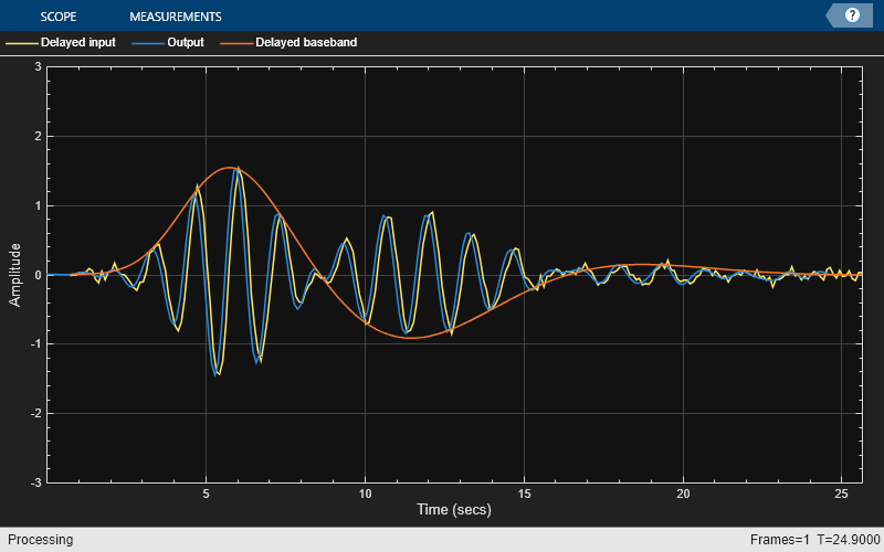
Carrier Shift and Phase Delay
Filter a modulated signal through the filter, and plot the input against the output with the appropriate delay. As expected, the delayed input appears synchronized with the output under the same envelope (the delayed baseband signal), but have a slight phase shift - the phase delay of the carrier signal.
ubase = f(n*Ts); % Baseband signal (evelope)

wc = 2*pi*Fc; % Carrier frequency
u  = f(n*Ts).*cos(wc*n*Ts) + 0.05*randn(size(n));
y  = g3(u);

ts = timescope(SampleRate=Fs,...
               TimeDisplayOffset=[D 0 D],...
               ChannelNames=["Delayed input" "Output" "Delayed baseband"],...
               YLimits=[-3 3]);

ts(u(1:250),y(1:250),ubase(1:250))
To obtain this phase delay , use the phasez function.
% phasez parses the first argument as a frequency whenever it is a vector
% of at least two elements. Therefore, we must pass [Fc Fc] instead of just Fc.
phi = phasez(g3,[Fc Fc],Fs);
pd  = -phi(1)/wc
pd =
0.6188
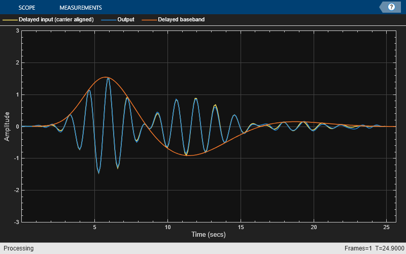
Use the phase delay to shift the carrier. Accounting for the phase delay, the filter output is almost perfectly aligned with the delayed input reference.
yref = f(n*Ts-D).*cos(wc*(n*Ts-pd));

ts = timescope(SampleRate=Fs, ...
               TimeDisplayOffset=[0 0 D],...
               ChannelNames=["Delayed input (carrier aligned)" "Output" "Delayed baseband"],...
               YLimits=[-3 3]);

ts(yref(1:250), y(1:250), ubase(1:250))
Using outputDelay with dsp.FilterCascade Objects
The outputDelay function can be used with filter cascade objects, even if they contain nonlinear phase stages (although this is a more nuanced case). For example, combine an IIR halfband interpolator, a lowpass filter, and a rational rate converter.
g5 = cascade(dsp.IIRHalfbandInterpolator(DesignMethod="Quasi-linear phase"), ...
                dsp.LowpassFilter(FilterType="IIR"), ...
                dsp.FIRRateConverter(7,4));
The input sample rate is either specified using the InputSampleRate argument or derived from the first stage of the dsp.FilterCascade object. If InputSampleRate is unspecified and the first stage does not have a sample rate property, the default sample rate is InputSampleRate = 1. In this case, the first stage is an IIR Halfband Interpolator, and its sample rate is 22.05 kHz.
FsIn = g5.Stage1.SampleRate
FsIn =
22050
The output sample rate expected in g5 is =77.175 kHz, which is indeed the output sample rate returned from outputDelay.
[D, FsOut] = outputDelay(g5,CarrierFrequency=0) % The input sample rate is of the first stageD = 18.8481
FsOut =
3.5000
Verify that the same result is obtained when you specify InputSampleRate = 22050.
[D, FsOut] = outputDelay(g5,InputSampleRate=FsIn,CarrierFrequency=0)
D =
8.5479e-04
FsOut =
77175
Process a signal through g5 and plot the results. The input and output are synchronized.
y = g5(u);
ts = timescope(SampleRate=[FsIn FsOut], ...
                TimeDisplayOffset=[0 -D],...
                ChannelNames=["Input" "Output"],...
                YLimits=[-3 3]);

ts(u(1:250),y(1:650))
The designRateConverter function sometimes returns multirate filter cascades in a dsp.FilterCascade System object. For example, design a sample rate converter from 192 kHz to 44.1 kHz and find its output delay and sample rate. The default filter designs used in designRateConverter are symmetric FIR filters. In other words, all stages have a linear phase and there is no need to specify Fc.
src = designRateConverter(InputSampleRate=192e3,OutputSampleRate=44.1e3)
src =
  dsp.FilterCascade with properties:

         Stage1: [1×1 dsp.FIRDecimator]
         Stage2: [1×1 dsp.FIRRateConverter]
    CloneStages: true
[D, FsOut] = outputDelay(src)
D =
4.6687e-04
FsOut =
44100
Band Measurement of dsp.FilterCascade Objects
For band measurement, the cascade must be reducible to a single filter stage using noble identities. For example, the cascade g5 can be reduced to have a single convolution stage. Measure the input band for that filter.
[D, FsOut, B] = outputDelay(g5,InputSampleRate=Fs,CarrierFrequency=0,Tolerance=0.1)
D =
1.8848
FsOut =
35
B = 1×2

   -1.1450    1.1450
If a cascade has a nonlinear stage and is not reducible, outputDelay will error out. For example an interpolator chained after a decimator is usually irreducible to a single filter cascade. Call outputDelay and note that it errors out.
g = cascade(dsp.FIRDecimator,g3,dsp.FIRInterpolator);
% >> [D,~,B] = g.outputDelay();
% Error using dsp.FilterCascade/outputDelay
% Analysis of multistage-multirate filters in which interpolators follow decimators is not supported unless the
% cumulative rate change factors of the interpolators is equal to the cumulative rate change factors of the decimators.
% The cascade is irreducible to a single stage, so band estimation is not supported.